
This function returns a subtotal for a range of data, typically used in lists or databases. While the Data > Subtotal command is often easier for creating subtotals, the SUBTOTAL() function allows for post-creation modifications.
Syntax:
SUBTOTAL(function_num; ref1; [ref2]; …)
Arguments:
- function_num (required)
- A number between 1–11 (includes hidden rows) or 101–111 (excludes hidden rows) that specifies the calculation method.
Table 1: Function Codes
| Code (Includes Hidden) | Code (Excludes Hidden) | Function |
| 1 | 101 | AVERAGE() |
| 2 | 102 | COUNT() |
| 3 | 103 | COUNTA() |
| 4 | 104 | MAX() |
| 5 | 105 | MIN() |
| 6 | 106 | PRODUCT() |
| 7 | 107 | STDEV() |
| 8 | 108 | STDEVP() |
| 9 | 109 | SUM() |
| 10 | 110 | VAR() |
| 11 | 111 | VARP() |
- ref1, ref2, …
- ref1 (required): The range to subtotal.
- ref2 (optional): Additional ranges (up to 254 total).
Key Features:
- Filters & Hidden Rows:
- Codes 1–11 include rows hidden manually (Format > Hide).
- Codes 101–111 exclude manually hidden rows.
- Always ignores rows filtered out (regardless of code).
- Nested Subtotals:
- Automatically skips other SUBTOTAL() results within the range to avoid double-counting.
- Limitations:
- Fails with 3D references (#VALUE! error).
- Designed for vertical ranges (columns). Hiding columns in horizontal ranges (e.g., =SUBTOTAL(109,B2:G2)) has no effect.
Example: Filtered Sum
Scenario: Calculate total sales for Michigan after filtering.
- Original Data (C2:C8):
=SUBTOTAL(9, C2:C8) // Sum all visible rows (includes hidden)
or
=SUBTOTAL(109, C2:C8) // Sum only non-hidden rows
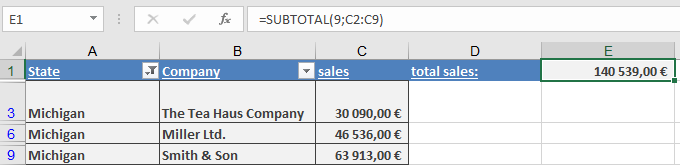
- After Filtering (Michigan):
- The result automatically updates to exclude filtered-out states.
Note: For dynamic reports, combine with Excel’s Filter or Table features.