How to use the COLUMN function in Excel

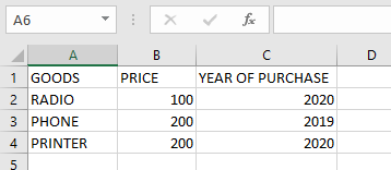
The COLUMN function returns the column number of a specified cell reference within a worksheet. This function provides the numerical position of a column in Excel’s grid system.

Syntax:

=COLUMN([reference])

Argument:

• reference (Optional):
  The cell or range for which you want to determine the column number.
  • If omitted, returns the column number of the cell containing the formula.

USING THE COLUMN FUNCTION

Example: Finding Column Numbers

To find the column number of cell A4:

1. Select a blank cell
2. Enter the formula:

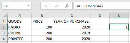
=COLUMN(A4)

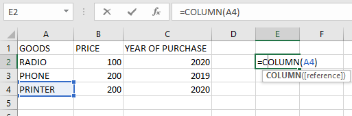
1. Press Enter and the column number will be displayed

To find the column number of cell B3:

1. Select a blank cell
2. Enter the formula:

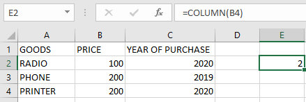
=COLUMN(B4)

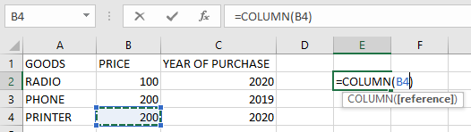
1. Press Enter → Returns 2 (B is the second column)

To find the column number of cell C1:

1. Select a blank cell
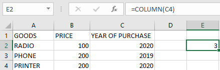
2. Enter the formula:

=COLUMN(C4)

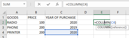
1. Press Enter → Returns 3 (C is the third column)

Using COLUMN without reference:

=COLUMN()

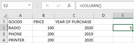
Returns the column number of the cell containing this formula.

IMPORTANT NOTES:

1. Single Reference Only:
   • Cannot process multiple cell references simultaneously
2. Reference Types Accepted:
   • Works with single cells or range references
   • Returns the leftmost column number for ranges
3. Optional Argument:
   • When omitted, automatically references the formula cell
4. Practical Applications:
   • Useful in combination with other functions like INDEX, OFFSET
   • Helps create dynamic column references in formulas