How to use the INDEX function in Excel

This function retrieves a value (or reference) from an array or cell range based on specified row and column indices.

Syntax (Array Version):

INDEX(array; row_num; [column_num])

Syntax (Reference Version):

INDEX(reference; row_num; [column_num]; [area_num])

Arguments

Array Version:

• array (required): A range of cells or an array constant (e.g., {1,2;3,4}).
• row_num (optional):
  • The row number to return (must be ≤ total rows).
  • Omit if array has only one row.
• column_num (optional):
  • The column number to return (must be ≤ total columns).
  • Omit if array has only one column.

Reference Version:

• reference (required): One or more cell ranges (use parentheses for multiple ranges: (A1:B2, C1:D2)).
• row_num, column_num (optional): Same as array version, but can reference non-contiguous areas.
• area_num (optional): Selects which range in reference to use (e.g., 1 for the first range).

Background

Array Version:

• Indices start at 1.
• Omitting row_num or column_num returns an entire column/row (use as an array formula).
• Errors:
  • #REF! if indices exceed the range.
  • #VALUE! if omitting arguments in non-array formulas.

Reference Version:

• Use parentheses for multiple ranges (e.g., (A1:B2, C1:D2)).
• area_num selects the nth range (default: 1).

Examples

1. Basic Array Usage:

• Return a single value:

=INDEX(B4:C6, 3, 2)  // Returns C6 (3rd row, 2nd column). 

• Array constant (columns separated by commas, rows by semicolons):

=INDEX({11,12,13; 21,22,23}, 2, 3)  // Returns 23. 

2. Array Formulas:

• Return entire column (3rd column):

{=INDEX({11,12,13; 21,22,23}; 0; 3)}  // Returns 13, 23 (vertical cells). 

• Return entire row (2nd row):

{=INDEX({11,12,13; 21,22,23}; 2; 0)}  // Returns 21, 22, 23 (horizontal cells). 

3. Reference Version:

• Multiple ranges:

=INDEX((B18:C20; E18:G19); 3; 2; 1)  // Returns C20 (3rd row, 2nd column in 1st range). 

• Named ranges:

=INDEX((FirstRange, SecondRange); 2; 1; 2)  // Returns E19 (2nd row, 1st column in SecondRange). 

4. Practical Applications:

• Searching Lists:

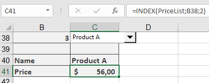
=INDEX(PriceList; B38; 1)  // Returns product name from row B38. 

=INDEX(PriceList; B38; 2)  // Returns price from row B38. 

  Finding information  

This example demonstrates the reference version of the function. Assume that you have divided an advanced training course into three parts and offer single-unit or complete conference reservations. You also offer an early-bird discount for participants who book before a deadline. The details are shown In the figure below.

To calculate the price based on the elements booked and the reservation date, you use the following formula:

=INDEX((D47:D50;E47:E50);VLOOKUP(C53;B47:C50;2;FALSE);;IF(C54<C52

;1;2))

• Dynamic Ranges: Sum last cells of two named ranges:

=INDEX(NumberOne; ROWS(NumberOne); COLUMNS(NumberOne)) + INDEX(NumberTwo; ROWS(NumberTwo); COLUMNS(NumberTwo)) 

Notes

• Use Ctrl+Shift+Enter for array formulas (legacy Excel).
• For dynamic ranges, combine with ROWS(), COLUMNS(), or OFFSET().