
Returns a dynamic reference to a range shifted by a specified number of rows/columns from a starting cell or range.
Syntax:
OFFSET(reference; rows; cols; [height]; [width])
Arguments:
| Argument | Required? | Description |
| reference | Yes | The anchor cell or range (e.g., A1 or B2:D5). Must be a valid reference. |
| rows | Yes | Number of rows to offset (positive = down, negative = up). |
| cols | Yes | Number of columns to offset (positive = right, negative = left). |
| height | No | Row count of the returned range. Defaults to reference’s height. |
| width | No | Column count of the returned range. Defaults to reference’s width. |
Background. This function doesn’t move cells on the worksheet; it moves the reference to a specified range. If you specify a value for the rows and columns arguments beyond the current sheet, the OFFSET() function returns the #REF! error.
The function expects integers for the four last arguments, and the last two integers must be positive. If the expressions in these arguments are evaluated to fractions, the decimal places are removed. No error occurs.
If you don’t specify the height and width arguments, Excel assumes that the new reference has the same height and width as the initial reference.
If the height argument is smaller than the height of the destination range, the remaining cells display the #N/A error. The same applies to the width argument. If the value is 1, the corresponding rows and columns are repeated in the remaining cells. As shows an example below.

The reference named MyRange has the dimensions two rows x three columns. The formula
{=OFFSET(MyRange;0;1;2;1)}
moves the target to the first cell in the range (B13) and offsets this by zero rows and one column, taking the starting point to cell C13. The height and width parameters extend the range to two rows and one column to target C13:C14. The destination range F13:I15 has the dimensions three rows x four columns. The destination range is filled with the values from C13:C14, repeating this four times across the destination range, but the remaining row
(15) is filled with the error #N/A.
Examples:
The following examples illustrate how the OFFSET() function is used.
Use this function to address single cells in the original named range. In this case, you don’t move the entire range but only the upper-left corner of the range. If you specify the value 1 for the height and width, the result is a single cell.
Assume that your range, MyRange, includes cells B5 through D6. Cell D6 is the last cell in the range and can be addressed with the array formula
{=OFFSET(MyRange;1;2)}
To move the required reference to the right or down, start at the upper-left cell of the range: two cells to the right and one cell down.
This method is especially useful if you use dynamic ranges, which change over time (for example, a dynamic list, a manually entered list, or a list updated with a database). In this case, use the COUNT() or COUNTIF() function to specify the position. This is explained in the following examples.
Assume that you have a list like the one shown in the table below. You want to filter the information in the list using database functions. The list constantly changes because records are added or removed.
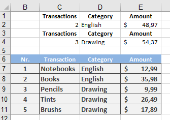
Create the data list in a worksheet named Calculations. The titles of the columns don’t have to match the list titles (for example, you could use Category instead of Categories).
Select the list titles. Select the Insert/Names/Define menu option or click Define Name in the Defined Names group on the
Formula tab. Enter the name list for the range defined by the following formula:
=OFFSET(Calculations!$B$6:$E$6;0;0;COUNT(Calculations!$B:$B)+1)
Based on the number of numeric entries in column B, the upper-left cell of the title range ($B$6:$E$6) is dynamically extended by the adjustable height argument. Remember that +1 is necessary to include the titles in the list.
You can now add up the invoice amounts in the English category using the following formula:
=DSUM(list;E6;D1:D2)
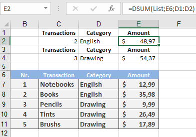
The DSUM() function takes the values identified by the list range and sums the values in the Amount column according to the criteria set in the range D1:D2 (Category, English). Other entries are evaluated with DCOUNT()
=DCOUNT(list;B6;D1:D2)
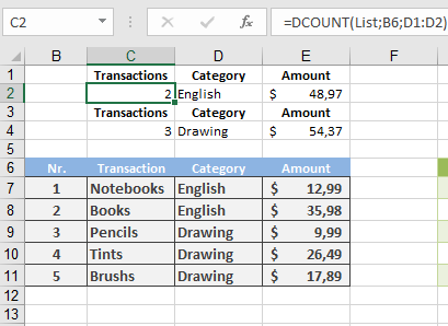
to return a count of the transaction. (The second argument can be empty.)
If you use Excel and format the list as a table, you don’t have to specify the range name. If the table has the name Table1 (the default name), the formula is
=DCOUNT(Table1[#All];B6;D1:D2)
You can use the method explained in the previous example to generate dynamic charts. Define a dynamic range name and use the named range to create the chart. Use a named range for the legend and data, as in these formulas:
=OFFSET(Charts!$C$4;0;Charts!$B$23)
=OFFSET(Charts!$C$5:$C$19;0;Charts!$B$23)
where the value in cell B23 defines which column should be selected to generate the chart.
Common Errors & Fixes:
| Error | Cause | Solution |
| #REF! | Offset outside sheet limits. | Adjust rows/cols or anchor point. |
| #N/A | Output range larger than height/width. | Ensure height/width ≥ destination range. |
| #VALUE! | Invalid reference (e.g., non-range). | Use a cell/range reference (e.g., A1). |
Alternatives to OFFSET():
- INDEX() + MATCH(): More efficient for static lookups.
- Excel Tables (Ctrl+T): Auto-expanding ranges without formulas.
- INDIRECT(): For text-based references (but volatile).