
This function returns TRUE if the value is the #N/A error. Otherwise, it returns FALSE.
Syntax
ISNA(value)
Arguments
- value (required) – The expression to check (a number, text, a formula without an equal sign, a logical value, an error value, a reference, or a name).
Background
- Part of the IS() function family, which evaluates arguments without conversion (e.g., numeric strings remain text).
- Specifically checks for the #N/A error, unlike ISERROR() (which detects all errors) or ISERR() (which excludes #N/A).
- Useful for error handling in lookup functions (VLOOKUP, HLOOKUP, MATCH, etc.).
Example: Handling #N/A in Lookups
Problem:
When using VLOOKUP(), a missing search term returns #N/A, which may disrupt reports or dashboards.
Solution:
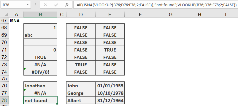
Replace #N/A with a custom message while allowing other errors to display normally:
=IF(ISNA(VLOOKUP(B76, D76:E78, 2, FALSE)), « Not found », VLOOKUP(B76, D76:E78, 2, FALSE))
How It Works:
- VLOOKUP(B76, D76:E78, 2, FALSE) searches for B76 in the range D76:D78.
- ISNA() checks if the result is #N/A:
- If TRUE → Returns « Not found ».
- If FALSE → Returns the lookup result (or other errors like #VALUE!).
Key Notes
- Precision: Only suppresses #N/A, preserving other errors (e.g., #REF!, #VALUE!) for debugging.
- Alternatives:
- Use IFERROR() to handle all errors (not just #N/A).
- Combine with IFNA() for cleaner syntax.
When to Use ISNA()
- Data Validation: Flag missing values without masking other errors.
- Conditional Formatting: Highlight cells with #N/A differently from other errors.