This function returns a number indicating the data type of the specified value.
Syntax: TYPE(value)
Arguments:
- value (required): The expression to check (a number, text, a formula without an equal sign, a logical value, an error value, a reference, or a name).
Background:
- The TYPE() function is related to the IS() functions, which return logical values based on the argument’s type.
- It is often used with IF() to pre-test calculation results, and its output can support conditional formatting and data validation rules.
- To use this function effectively, refer to the mappings in Table 1.
Table 1. Data Types Mapped to Numbers
| Argument | Return Value |
| Number | 1 |
| Text | 2 |
| Logical value | 4 |
| Error value | 16 |
| Array | 64 |
Key Notes:
- Except for arrays, the results can also be obtained using ISNUMBER(), ISTEXT(), ISNONTEXT(), ISLOGICAL(), and ISERROR(). For example:
- ISNUMBER(B12) and TYPE(B12) = 1 are logically equivalent.
- Limitations:
- ISBLANK(), ISNA(), ISREF(), and ISERR() (which excludes #N/A) are incompatible with TYPE().
- TYPE() cannot detect whether a cell contains a formula—it only returns the result’s data type.
- For array formulas, TYPE() returns 64 only if the argument is a range entered with Ctrl+Shift+Enter.
Examples:
- Replicating IS() Functions:
- Replace =ISERROR(B3) with =(TYPE(B3)=16).
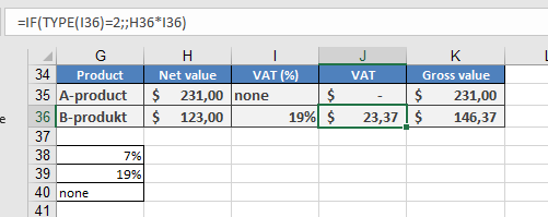
- Replace =IF(ISTEXT(I36);;H36*I36) with =IF(TYPE(I36)=2;;H36*I36).