Structured References in Excel Tables

One of the most powerful and practical features of Excel tables is the use of structured references. At first glance, this special syntax for referencing table data may appear complex or even confusing, especially if you’re accustomed to traditional cell references. However, once you begin to work with it, you’ll quickly discover how useful and efficient this functionality can be—especially in dynamic data environments.

A structured reference, also known as a table reference, is a specific way to refer to parts of an Excel table by using the table’s name and column headers, rather than standard cell addresses like A1 or B2. This makes formulas easier to read, more intuitive, and more resilient to changes.

The reason this type of referencing is so essential lies in the inherent power of Excel tables: unlike regular cell ranges, tables automatically expand or contract when data is added or removed. Standard cell references do not adapt to these changes, which can lead to inaccurate results or broken formulas. Structured references, on the other hand, dynamically adjust to include new rows or columns, ensuring that your formulas always remain up to date.

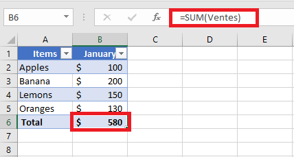
For instance, to sum the values from cells B2 to B5 using a regular cell range, you would write:

=SUM(B2:B5)

But if your data is organized in an Excel table named SalesTable, and you want to sum the values in the « Sales » column, you would use a structured reference like this:

=SUM(SalesTable[Sales])

This formula is not only easier to interpret (you know exactly what it sums), but it will also automatically include any new sales data added to the table.

Key Features of Structured References in Excel

Compared to standard cell references, structured references offer several advanced features that enhance both the flexibility and efficiency of working with data in Excel tables:

■ Easy to Create
Structured references are incredibly simple to insert into a formula. You don’t need to memorize any special syntax—just select the desired table cells with your mouse, and Excel automatically generates the correct structured reference. This makes it accessible even to users unfamiliar with the syntax.

■ Automatically Resilient and Self-Updating
One of the greatest advantages of structured references is their ability to automatically adapt to changes. When you rename a column in a table, all associated structured references are immediately updated to reflect the new column name—eliminating the risk of broken formulas. Furthermore, when you add new rows to the table, those rows are seamlessly included in existing references, ensuring that formulas always cover the entire data range.

This means that no matter how frequently your data changes, your structured references remain accurate and up to date, reducing the need for manual adjustments.

■ Usable Both Inside and Outside the Table
Structured references are not limited to formulas within the table itself. You can also use them in formulas located outside the table, which is especially helpful in large workbooks where you may need to reference specific tables from various sheets. This improves clarity and makes it easier to manage complex spreadsheets.

■ Auto-Fill for Calculated Columns
When you enter a formula in a single cell of a table column, Excel automatically fills the rest of the column with the same formula—creating what’s known as a calculated column. This feature ensures consistency in your computations and saves time by applying the formula to all rows without manual copying.

How to Create a Structured Reference in Excel

Creating a structured reference in Excel is both straightforward and intuitive. If you’re starting with a regular range of data, your first step should be to convert that range into an official Excel table. This unlocks all the advanced features of table management, including structured references.

To convert a standard data range into a table:

• Select the entire dataset.

• Press Ctrl + T (or Ctrl + L in some older versions of Excel).

• Make sure the « My table has headers » option is checked, then click OK.

Once your data is formatted as an Excel table, you can create structured references by following these simple steps:

• Begin writing your formula
  Start as usual by typing the equals sign (=) in the desired cell.
• Select the relevant cells in the table
  Instead of typing cell addresses, simply use your mouse to select the cell or range you want to include from within the table. Excel will automatically insert the structured reference using the table name and column headers. This eliminates the need to know the syntax by heart.
• Close the formula and press Enter
  Once your structured reference is inserted, complete the formula by typing the closing parenthesis ) and pressing Enter. If you’re entering the formula inside the table, Excel will automatically fill the entire column with the same formula, creating a calculated column.

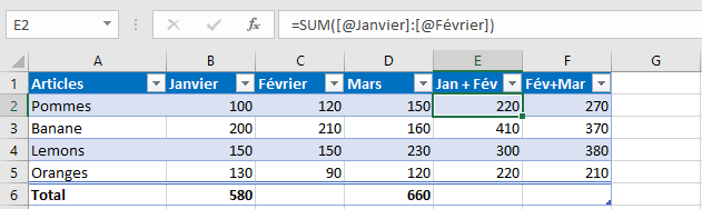
Example: Summing Monthly Sales
Suppose you have a table named MonthlySales, and it contains sales figures for three months across columns B, C, and D. You want to calculate the total sales per row in column E.

To do this:

• Click in cell E2 (the first row of your total column).

• Type: =SUM(

• Select the cells B2 to D2 (Excel will translate this into a structured reference like =SUM(Article[@[January]:[March]]) depending on your column headers).

• Type the closing parenthesis ) and press Enter.

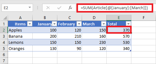
As a result, the entire column E is automatically filled with the following formula:
=SUM(MonthlySales[@[January]:[March]])

Even though the formula looks identical across all rows, Excel evaluates it individually for each row using the respective data. This row-wise behavior is one of the most powerful aspects of structured references in Excel tables.

Creating Structured References Outside of a Table

If you’re entering a formula outside of the table and only need to refer to a specific column or range of data within the table, you can quickly create a structured reference without manually selecting the cells. Here’s how:

• Begin typing the formula normally.
  For example, to calculate the maximum value in a column, you might start typing =MAX(.
• Type the first few letters of the table name.
  As soon as you type the first letter, Excel will display a dropdown list of all table names that match what you’re typing. The more letters you type, the more refined the list becomes.
• Use the arrow keys to select the correct table.
  Scroll through the list using the up/down arrow keys on your keyboard.
• Press Tab or double-click to insert the table name.
  Once the correct table is selected, press Tab or double-click the name to insert it into your formula.
• Complete the formula and press Enter.
  Add any column reference or closing parentheses needed and press Enter.

Example:
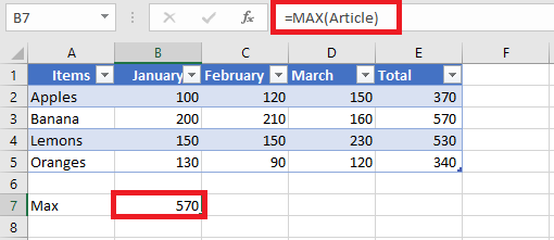
Let’s say you want to find the highest value in a table named Article.

• You begin by typing =MAX(

• Then type “Ar”

• Excel shows Article as a suggestion

• Press Tab to select it

• Complete the formula with ) and hit Enter

Your final formula looks like this:
=MAX(Article)

Structured Reference Syntax in Excel

As previously mentioned, you don’t necessarily need to master the syntax of structured references to use them in formulas—Excel inserts them automatically as you work with tables. However, understanding this syntax will help you interpret what your formulas are actually doing, especially when analyzing or debugging them.

In general, a structured reference is a text string that starts with the table name and ends with one or more column specifiers. To illustrate, let’s break down the following formula which adds the values from the “South” and “North” columns in a table named Regions:

This structured reference contains three main components:

• Table name

• Item specifier

• Column specifier(s)

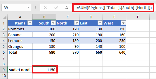
When you select the cell containing this formula and click into the formula bar, Excel highlights the exact cells involved in the calculation, helping you visualize the data being referenced.

Table Name

The table name refers only to the data body of the table—it excludes both the header row and the total row. This name may be the default (e.g., Table1) or a custom name like Regions.
If your formula is located inside the same table, Excel often omits the table name because it is implicitly understood.

Column Specifier

A column specifier refers to the data within a specific column, excluding the header and total rows. It is written inside square brackets.
For example:

To reference multiple adjacent columns, you can use a range operator (colon), like this:

If a column name contains spaces, punctuation, or special characters, Excel adds an extra set of square brackets:

Item Specifier

To reference specific parts of a table (such as the entire table or just the headers), Excel uses item specifiers. These always begin with a hash symbol (#) except for row-specific references using @.

Structured Reference Operators

Structured references support various operators that enhance their flexibility:

• Range Operator (:)

Used to reference a range of adjacent columns. For example:

This sums the current row’s values from “South” to “West”.

• Union Operator (, comma)

Used to reference non-adjacent columns. For instance:

This adds values from the “South” and “West” columns in the same row.

• Intersection Operator ( space)

Used to refer to the value at the intersection of a specific row and column. For example, to return the value at the intersection of the Total row and the West column:

Note: In this case, the [#All] specifier (or a similar item specifier) is essential, because column specifiers alone do not include the total row. Without it, Excel may return a #NULL! error.

Syntax Rules for Structured Table References

When manually editing or creating structured references in Excel tables, it’s important to follow specific syntax rules to ensure formulas work properly and remain readable. Below are the main guidelines to follow:

Enclose Specifiers in Brackets
All column specifiers and special item identifiers must be enclosed in square brackets [ ]. If a specifier includes multiple elements or a range, it should be wrapped in an additional set of brackets.
Example:
To reference a range from the “South” column to the “West” column in the current row:
=Regions[@[South]:[West]]

Separate Multiple Specifiers with Commas or Semicolons
When combining two or more inner specifiers within a single reference, separate them with commas (, in English versions) or semicolons (; in French versions), depending on your regional Excel settings.
Example:
To reference the column header for « South » within a structured reference, use an additional set of brackets and separate specifiers:
=Regions[[#Headers],[South]]

Do Not Use Quotation Marks Around Column Headers
In structured references, column headers should not be enclosed in double quotes—even if they contain text, numbers, or dates. Excel automatically interprets them based on the table’s metadata.

Use Single Quotes for Special Characters in Column Headers
Certain characters within column headers—such as square brackets [ ], the pound/hash symbol #, and the single quote '—have special meaning in Excel. If one of these appears in a column name, precede it with a single quote (') within the reference to avoid syntax errors.
Example:
If a column is named Item #, you must escape the # with a single quote:
=Regions[[#Headers],[Item '#]]

Use Spaces to Improve Readability
While not mandatory, inserting spaces between specifiers (especially after commas or semicolons) improves the clarity and readability of complex structured references.
Example:
To average the values in columns “South”, “North”, and “West” from the current row, you can use:
=AVERAGE(Regions[@[South]]; Regions[@[North]]; Regions[@[West]])

Structured References in Excel Tables

To better understand how structured references work in Excel tables, let’s review a few practical and illustrative examples. These examples are designed to be simple, meaningful, and applicable to real-world scenarios.

Counting Rows and Columns in an Excel Table

To determine the number of columns or rows in a table, you can use the built-in Excel functions COLUMNS and ROWS, which only require the table name as input:

These formulas return the total number of columns and data rows in the table named Sales.

If you want to include both the header row and the Total Row (if present), use the special item specifier [#All]:

=ROWS(Sales[#All])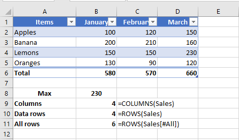

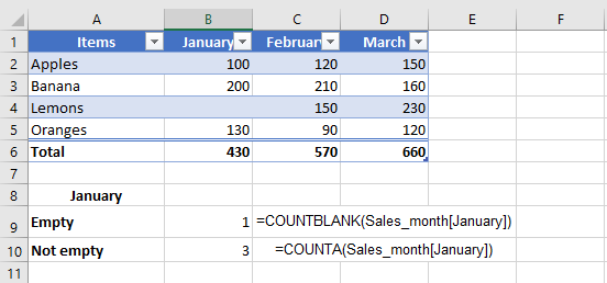
This will return the number of all rows including the header and total rows.

Counting Blank and Non-Blank Cells in a Specific Column

When working with a specific column in a table, you may want to count how many cells are empty or contain data. Be sure to place your formula outside of the table to avoid circular references and incorrect results.

• To count blank cells:

• To count non-blank cells:

If your table is filtered and you want to count only the non-blank cells in the visible rows, use the SUBTOTAL function with function number 103:

This version of the formula ignores filtered-out (hidden) rows and only counts visible non-empty cells.

Summing Values in an Excel Table

The fastest way to calculate totals in an Excel table is by enabling the Total Row option:

• Right-click anywhere inside the table.

• Select Table from the context menu.

• Click Total Row.

Excel will add a summary row at the bottom of the table. By default, it may only calculate the total for the last column, leaving the rest empty.

To fix this, click any empty cell in the Total Row, click the dropdown arrow that appears, and choose the SUM function. Excel will insert a structured SUBTOTAL formula that adds only the values from visible rows, ignoring any filtered-out data:

Likewise, a regular SUM function using a structured reference (e.g., =SUM(Sales[January])) won’t work inside the table for the same reason.

Relative and Absolute Structured References in Excel

By default, structured references in Excel tables behave according to specific rules, which can impact how formulas respond when copied or dragged across cells:

• References to multiple columns are absolute by nature. They do not change when the formula is copied or moved across the worksheet.

• References to a single column are relative when formulas are dragged horizontally across columns, meaning the column reference will adjust. However, when such formulas are copied and pasted using standard commands (Ctrl+C and Ctrl+V), the references remain fixed.

This behavior presents a challenge when you need a combination of relative and absolute references in your table formulas. Dragging a formula will shift single-column references (which may be undesired), while copying and pasting will fix all references (removing the intended dynamic behavior). Fortunately, there are practical tricks to control this behavior precisely.

Absolute Structured Reference to a Single Column

To force a single-column reference to behave like an absolute reference, repeat the column name to explicitly define it as a range.

• Relative column reference (default):
  TableName[Column]

• Absolute column reference:
  TableName[[Column]:[Column]]

To refer to the current row with an absolute column reference, use the @ symbol before the column name:

• TableName[@[Column]:[Column]]

Example Use Case

Imagine you want to sum the monthly sales of a specific product over three months. You enter the product name in cell F2, and use the SUMIF function to calculate the total sales for January:

However, if you drag this formula to the right to calculate totals for February and March, the [Items] reference might shift, breaking the formula.

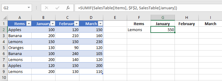
To prevent this, make the [Items] reference absolute while keeping [January] relative:

=SUMIF(SalesTable[[Items]:[Items]], $F$2, SalesTable[January])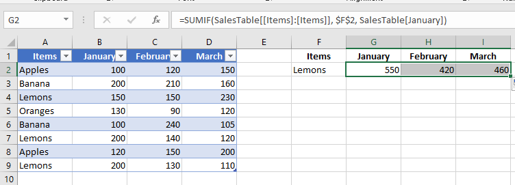

Now, when you drag the formula to adjacent columns, only the third argument (SalesTable[January]) updates accordingly (to February, March, etc.), while the [Items] column remains fixed.

Relative Structured References to Multiple Columns

By default, multi-column structured references in Excel tables are absolute and do not change when copied across cells. This default behavior is generally consistent and expected.

However, if you want to create a relative multi-column structured reference, you can do so by prefixing each column with the table name and removing the outer brackets.

• Absolute range reference (default):
  TableName[[Column1]:[Column2]]

• Relative range reference:
  TableName[Column1]:TableName[Column2]

To reference multiple columns in the current row, use the @ symbol with each column:

• @[Column1]:[Column2]

Example: Row-Level Summation

To sum the values in the current row for columns January and February, use:

This reference is absolute, so copying it to another column will still sum January and February.

If you want the referenced columns to adjust relative to the formula’s position, use a relative structured reference like this:

=SUM(Table10[@February]:Table10[@March])


Note that if the formula is written inside the same table, the table name (Table10) is optional and usually omitted by Excel automatically.