Once you’ve created a table in Excel, the first thing you’ll likely want to do is make it visually appealing and easy to interpret. Thankfully, Microsoft Excel offers a wide array of built-in table styles that allow you to instantly format or reformat a table with just one click. And if none of the default styles meet your specific design preferences, you can quickly define your own custom style.
Moreover, Excel allows you to toggle key table elements on or off — such as the header row, banded rows, total row, and more — giving you full control over the appearance and behavior of your table.
Built-in Table Styles
Excel tables are designed not just for data storage but for enhanced data management. They offer features like built-in filtering and sorting, calculated columns, structured references, and automatic total rows. When you convert a regular data range into a table, Excel automatically applies default formatting: alternating row colors (banded rows), border lines, and font styling.
If you’re not satisfied with the default format, you can easily change it via the Design tab that appears under Table Tools when a cell in the table is selected.
Example: Over 50 Built-in Table Styles
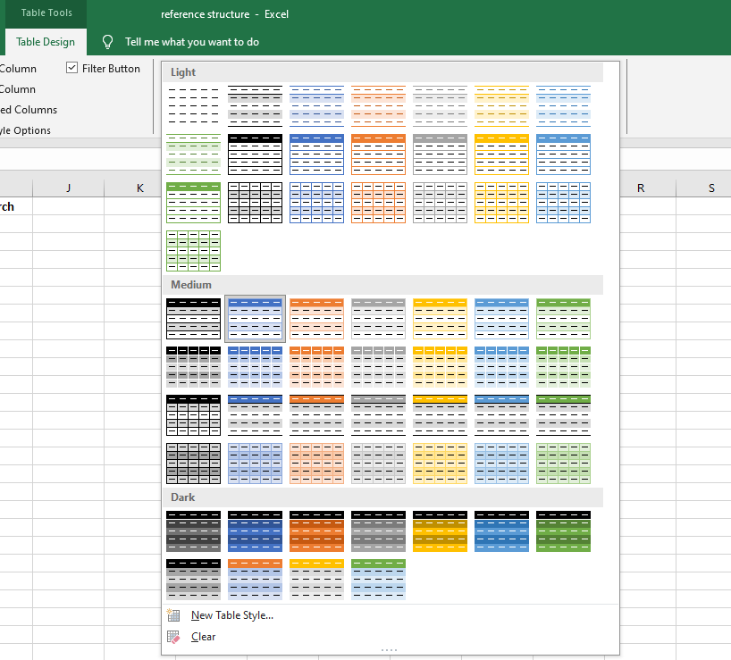
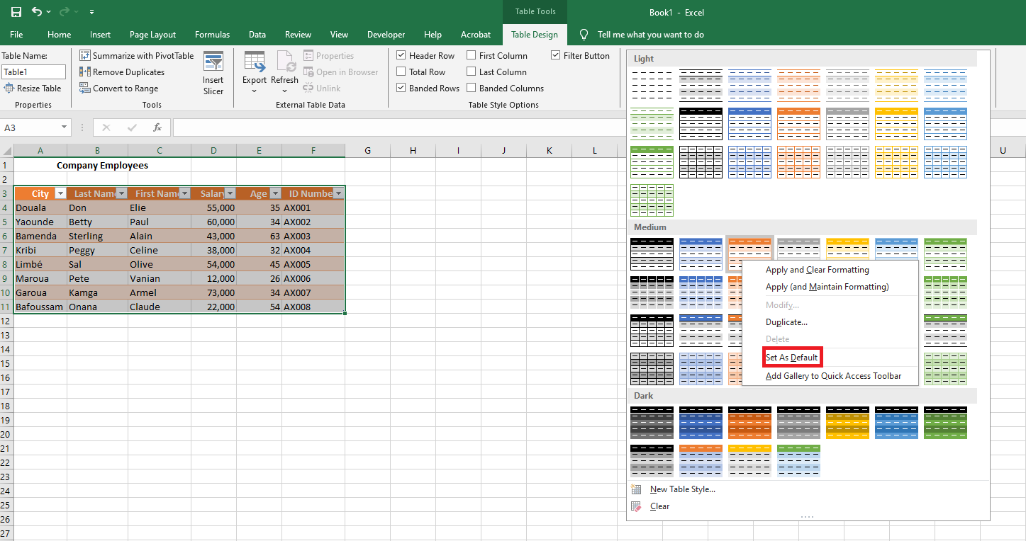
As shown in the illustration (Fig. 3.2.1.a), Excel provides a gallery of over 50 pre-defined styles, categorized as Light, Medium, and Dark themes. A table style acts as a formatting template, automatically applying visual elements to headers, rows, columns, and the total row.
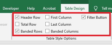
You can further customize your table using the Table Style Options, which allow you to control the appearance of specific elements:
-
Header Row – Show or hide the table headers.
-
Total Row – Add a summary row at the bottom of the table, with built-in functions for each column.
-
Banded Rows / Columns – Alternate shading for improved readability.
-
First/Last Column – Apply special formatting to highlight these columns.
-
Filter Button – Show or hide the dropdown filter arrows in the header row.
Choosing a Table Style While Creating a Table
To create a table and immediately apply a specific style, follow these steps:
-
Select the cell range you want to convert into a table.
-
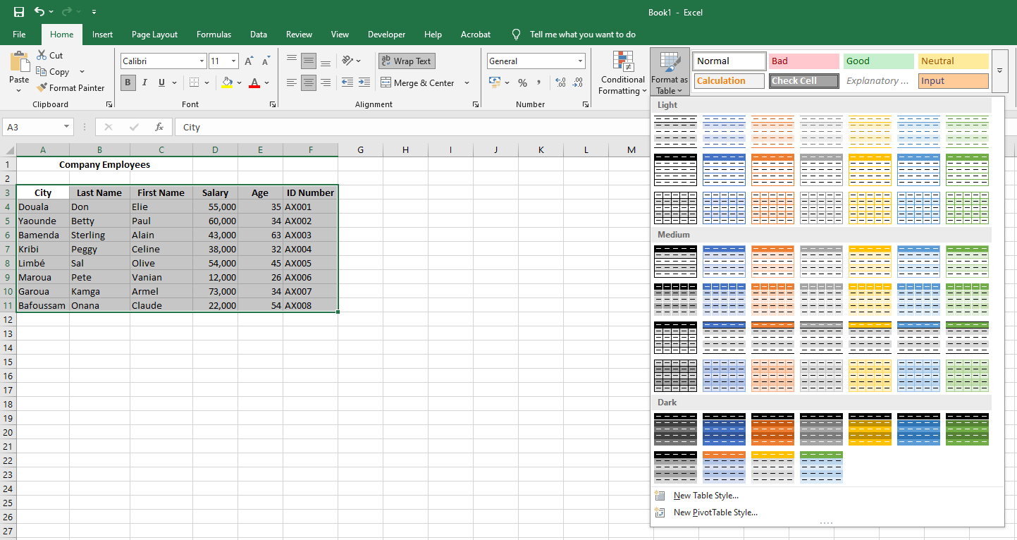
On the Home tab, go to the Styles group, and click Format as Table.
-
In the style gallery, click the table style you want to use.
Changing the Style of an Existing Table
To change the appearance of a table that already exists:
-
Click any cell inside the table.
-
Go to the Design tab under Table Tools, and in the Table Styles group, click the More arrow to see all available styles.
-
Hover over a style to preview it live on your table. Click to apply it.
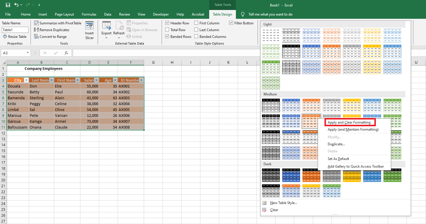
Tip: If you previously applied custom formatting (like bold fonts or custom colors) manually to some cells, Excel will retain them even when you switch styles. To override this and apply the new style completely, right-click the style and choose Apply and Clear Formatting.
5.4 Setting a Default Table Style for a Workbook
If you want every new table in your workbook to follow a specific style, set it as the default:
-
In the Table Styles gallery, right-click your preferred style.
-
Select Set As Default.
From now on, every table inserted via the Insert tab will adopt this style automatically.
Applying Table Styles Without Creating an Actual Table
If your goal is to quickly style a data range without converting it into a structured Excel table, here’s a workaround:
-
Select the data range you wish to format.
-
On the Home tab, in the Styles group, click Format as Table, then choose your desired style.
-
After the table is created, go to the Design tab and click Convert to Range to revert it back to a regular range.