Conditional formatting is a powerful feature when it comes to applying different formats to data that meets certain conditions. It helps highlight key information in your worksheets and quickly spot discrepancies in cell values at a glance.
At the same time, conditional formatting is often seen as one of the most complex and obscure Excel functions, especially by beginners. If you feel intimidated by this feature—don’t be! In reality, conditional formatting in Excel is quite simple and easy to use, and you’ll be convinced of that in just 5 minutes after reading this short tutorial.
Basics of Excel Conditional Formatting
Just like standard cell formatting, you use conditional formatting in Excel to style your data by changing fill color, font color, and cell border styles. The difference is that conditional formatting is more flexible—it lets you format only the data that meets specific criteria or conditions.
You can apply conditional formatting to one or more cells, rows, columns, or entire tables based on the content of the cell itself or based on the value of another cell. To do this, you create rules, which define when and how the selected cells should be formatted.
To get started, here’s where to find the conditional formatting feature in various versions of Excel. The good news is that in all modern versions of Excel, it’s located in the same place: Home tab > Styles group.

Now that you know where to find the feature, let’s move on and look at the formatting options and how to create your own rules.
Creating Conditional Formatting Rules
To take full advantage of conditional formatting, you’ll need to learn how to create different types of rules. These rules determine:
- Which cells the formatting should apply to
- What condition(s) must be met
Let’s walk through how to apply conditional formatting in Excel 2010 (features are similar across all versions):
- In your worksheet, select the cells to format.
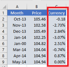
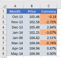
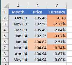
In this example, we’ll highlight all negative values (price drops) in the “Change” column. So, we select cells C2:C9.
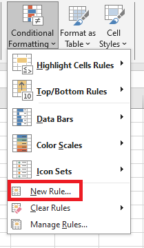
- Go to the Home tab > Styles group, then click Conditional Formatting.
You’ll see options like Data Bars, Color Scales, and Icon Sets. - Since we want to highlight numbers less than 0, choose Highlight Cells Rules > Less Than…
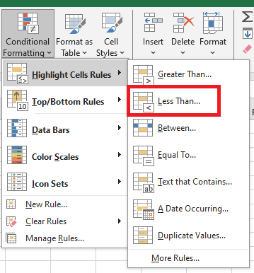
- Other useful rule types include:
- Format values greater than, less than, or equal to a certain number
- Highlight cells containing specific text or characters
- Highlight duplicates
- Format specific dates
- In the dialog box that appears, enter the value 0 under Format cells that are LESS THAN. Excel will instantly highlight all cells in the selected range that meet the condition.
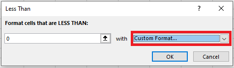
- Select the desired format from the dropdown, or click Custom Format…
- In the Format Cells window, use the Font, Border, and Fill tabs to define your style.
You’ll see a live preview. - Click OK to apply the rule.
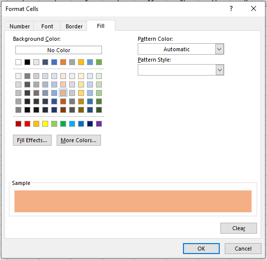
Tip: To access more fill or font colors, click More Colors… in the Font or Fill tab. To apply a gradient background, use Fill Effects.
Create a Custom Rule from Scratch
If none of the default rules meet your needs, you can create one from scratch:
- Select the cells, click Conditional Formatting > New Rule.
- In the dialog, choose a rule type. For example, “Format only cells that contain” and select between 103 and 104.9.
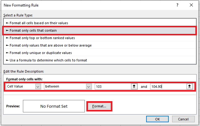
- Click Format… to choose styles.
- Click OK twice to apply the rule.
Format Based on Another Cell’s Value
Instead of typing a number in the rule, you can base it on another cell’s value. This is dynamic—when the referenced cell changes, the formatting updates automatically.
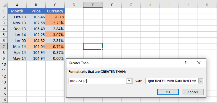
Example: In the “Oil Prices” table, highlight all prices in column B that are higher than the price in B5 (February).
Use Conditional Formatting > Highlight Cell Rules > Greater Than…, and select B5 instead of entering a number.
This is a simple example. For more complex scenarios, use formulas—explained in the article: How to change a cell color based on another cell’s value.
Apply Multiple Conditional Formatting Rules
You’re not limited to one rule per cell. You can apply several rules to the same cell/table.
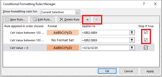
Example: In a weather table, shade temperatures:
- Above 102 in yellow
- Above 104 in orange
- Above 105 in red
Steps:
- Create the rules with Highlight Cell Rules > Greater Than…
- Go to Conditional Formatting > Manage Rules
- Use the arrows to set rule order (priority)
- Check Stop If True for the first two rules to prevent overlap
Use « Stop If True » in Rules
We used Stop If True above to stop lower-priority rules once a condition is met.
Two useful examples:
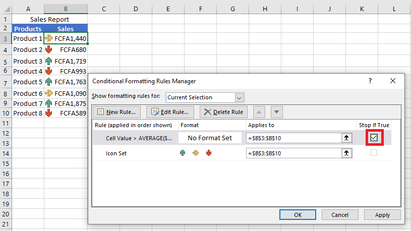
Example 1: Show Only Down Arrows in Icon Set
Suppose you apply an icon set (arrows) to your sales report:
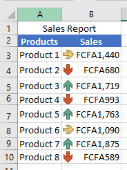
You want to keep only red down arrows for underperformers.
Steps:
- Create a rule: New Rule > Format only cells that contain
- Use the formula
=A2>AVERAGE($A$2:$A$10)(adjust cell refs)
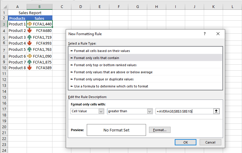
- Leave formatting blank.
- Go to Manage Rules, and check Stop If True for the new rule.
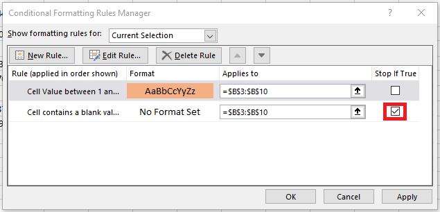
Example 2: Exclude Blank Cells from Formatting
You create a rule like “Between $0 and $1,000”, but empty cells also get highlighted.
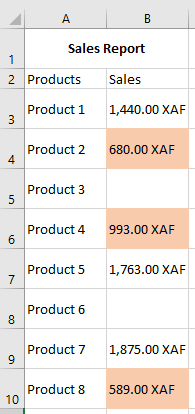
Fix it by:
- Creating a new rule: Format only cells that contain
- Choose Blanks
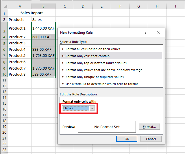
- Leave formatting blank, click OK
- In Manage Rules, check Stop If True next to the blank rule
Edit Conditional Formatting Rules
To edit an existing rule:
- Select a cell with the rule
- Click Conditional Formatting > Manage Rules
- In the Rules Manager, select the rule and click Edit Rule
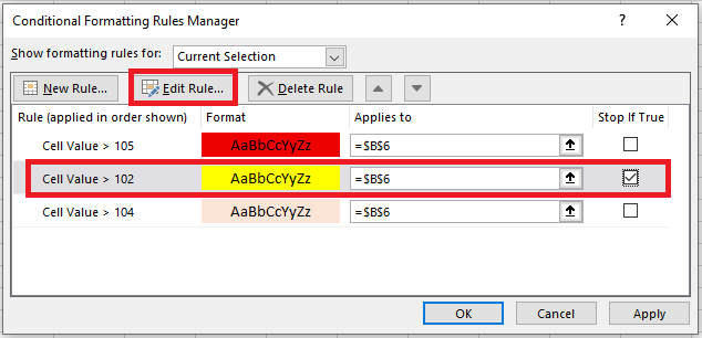
- Make changes and click OK
If you don’t see your rule, select This Worksheet in the dropdown at the top of the Rules Manager.
Copy Conditional Formatting
To apply a rule from one range to another:
- Click a cell with the rule
- Click Home > Format Painter (mouse turns into a brush)
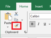
- Drag across the new range to apply formatting
- Press Esc to exit the tool
Note: If your rule uses formulas, you may need to adjust cell references afterward.
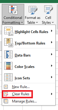
Delete Conditional Formatting Rules
Easiest part
To delete a rule:
- Open Conditional Formatting > Manage Rules, select the rule, click Delete Rule
- Or select the range, go to Conditional Formatting > Clear Rules, and pick from the options
You now have a solid understanding of basic Excel conditional formatting. In the next article, we’ll cover advanced features to push conditional formatting even further in your spreadsheets.