A simple way to change the appearance of a chart is to apply one of the built-in layouts or styles available in Excel.
Apply a Chart Layout
Built-in chart layouts quickly adjust the overall layout of a chart by combining titles, labels, and orientations.
-
Select the chart you want to format.
-
Click the Design tab.
-
Click the Quick Layout button.
-
Choose a layout from the list.
 The selected layout is applied to the chart.
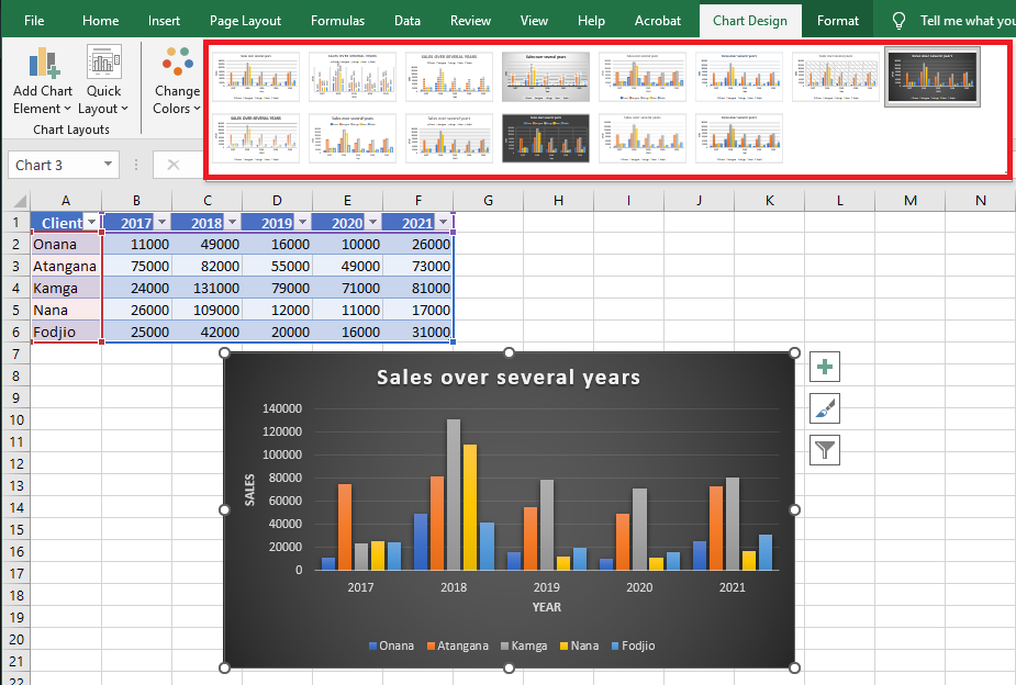
Apply a Chart Style
Built-in chart styles allow you to adjust the format of multiple chart elements at once.
Styles quickly change colors, shading, and other formatting properties.
-
Select the chart.
-
Click the Design tab.
-
Click the More Chart Styles button.
If the style you want is already shown in the gallery, you don’t need to expand the menu—just click to apply it. - Select a new style.
The new style is applied to the chart.
Change the Chart Colors
You can keep the overall style while updating only the colors to better suit your needs.
-
Select the chart.
-
Click the Design tab.
-
Click the Change Colors button.
- Select a new color palette.

The new color scheme is applied to the chart.
NOTE:
You can also access chart styles and colors using the Chart Styles icon (paintbrush) that appears to the right of the chart when selected.
The dropdown list shows the same choices as in the Chart Tools / Design / Chart Styles group.