
This function returns values along a linear trend. TREND() fits a straight line (using the least squares method) to the arrays of known_y’s and known_x’s. It then returns the corresponding y-values along that line for the specified array of new_x’s.
Syntax. TREND(known_y’s; known_x’s; new_x’s; const)
Arguments
known_y’s (required): The known y-values in the equation y = mx + b:
— If the known_y’s array is a single column, each column in known_x’s is treated as a separate variable.
— If the known_y’s array is a single row, each row in known_x’s is interpreted as a separate variable.
known_x’s (optional): The known x-values in the equation y = mx + b:
— This array may contain one or more sets of variables. If there’s only one variable, known_y’s and known_x’s can be ranges of any shape as long as they have matching dimensions. If there is more than one variable, known_y’s must be a vector (a single row or column).
— If known_x’s is omitted, it defaults to the array {1, 2, 3, …} with the same number of elements as known_y’s.
— known_y’s and known_x’s must have the same number of rows or columns. A mismatch leads to a #REF! error. A zero or negative y-value will produce a #NUM! error.
new_x’s (optional): The new x-values for which you want the function to return the corresponding y-values:
— Like known_x’s, new_x’s must have one column (or row) for each independent variable. If known_y’s is a single column, then known_x’s and new_x’s must have the same number of columns. If known_y’s is a single row, then known_x’s and new_x’s must have the same number of rows.
— If new_x’s is not provided, it is assumed to be equal to known_x’s.
— If both known_x’s and new_x’s are omitted, Excel assumes them to be {1, 2, 3, …} with the same number of elements as known_y’s.
const (optional): A logical value that specifies whether to force the constant b to equal 1:
— If const is TRUE or omitted, b is calculated normally.
— If const is FALSE, b is set to 1, and the slope m is adjusted so the formula becomes y = m^x.
Background
When you know that some values are interdependent, you can use TREND() to make predictions based on known data.
Excel provides several statistical functions for calculating trends. These functions determine a line or curve from existing values. By extending the timeline, you can forecast future values. Known values are analyzed and expressed as a formula for extrapolation. However, your dataset must be large enough to account for seasonal patterns. Unpredictable influences can also distort trend predictions.
Example: Suppose a competitor launches a highly successful new product in your area. This sudden change could disrupt your data model. Since regression analysis approximates data using mathematical functions, Excel includes various tools for this, including the TREND() function.
Use TREND() to identify a linear trend or analyze existing data. The values are plugged into a formula to help you forecast future changes.
The x- and y-values come from the equation y = mx + b, where:
— b is the y-intercept (where the line crosses the y-axis), and
— m is the slope (the rate of change of y for every unit change in x).
If changes follow a consistent pattern, a linear trend exists.
Example
You’re the marketing manager of a software company analyzing web traffic. Recently, both visits and online orders have significantly increased. You want to forecast future activity, so you use the TREND() function to project future values.
The website visits and orders up to June 2008 are shown in Figure below.

You generate a chart from the available data to visualize the linear trend for website visits and online orders. The chart includes equations and the coefficient of determination (r²), as shown in Figure below.
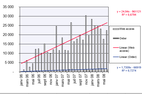
The linear trend line and equation show that orders increase by 52.872 each month — roughly 53 new orders per month.
You now want to project the trend for visits and orders from July 2008 to March 2009.
To calculate website visits over the next nine months, use these TREND() arguments:
- known_y’s = website visits from January 2008 to June 2008
- known_x’s = months from January 2006 to June 2008
- new_x’s = months from July 2008 to March 2009
- const = TRUE (calculate b normally in the equation y = mx + b)
Figure below displays the results.

By applying the same method, you can forecast online orders using the projected website visits. Figure below shows the calculated values and the arguments used in the TREND() function.
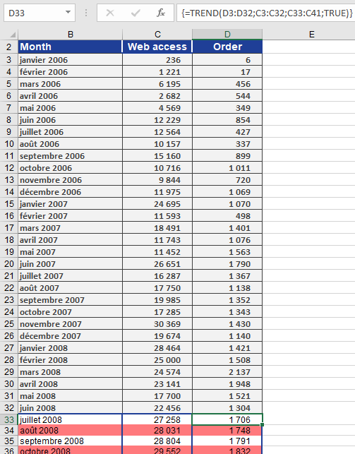
With the TREND() function, Excel allows accurate forecasting of website visits and online orders, assuming the previous exponential growth trend continues.