Absolute, Relative, and Mixed Cell References in Excel

A worksheet in Excel is made up of cells. These cells can be referenced by specifying the row number and column letter. For example, A1 refers to the first row (indicated by 1) and the first column (indicated by A). Likewise, B3 refers to the third row and the second column.

The power of Excel lies in the fact that you can use these cell references in other cells when creating formulas. There are three types of cell references that you can use in Excel:

• Relative cell references
• Absolute cell references
• Mixed cell references

Understanding these different types of cell references will help you work more efficiently with formulas and save time (especially when copying and pasting formulas).

Relative Cell References

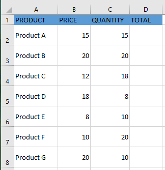
Let’s take a simple example to explain the concept of relative cell references in Excel. Suppose we have the following data set:

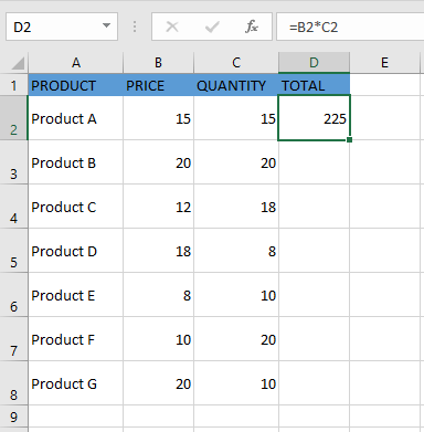
To calculate the total for each item, we need to multiply the price of each item by its quantity. For the first item, the formula in cell D2 would be =B2*C2 (as shown below):

Now, instead of entering the formula for each cell individually, you can simply copy the formula from cell D2 and paste it into all the other cells (D3:D8) using the fill handle. When you do this, you’ll notice that the cell references adjust automatically to refer to the corresponding rows. For example, the formula in D3 becomes =B3*C3, and in D4, it becomes =B4*C4.

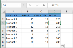
These cell references that adjust when the formula is copied are called relative references in Excel. Relative cell references are useful when you want to create a formula for a range of cells and have the reference adjust automatically for each row or column. In such cases, you can create the formula once and copy-paste it across the range.

Absolute Cell References

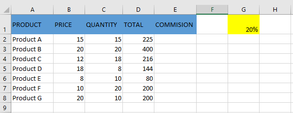
Unlike relative references, absolute cell references do not change when you copy the formula to other cells. For example, suppose you have the dataset below and need to calculate the commission for the total sales of each item. The commission rate is 20% and is listed in cell G1.

To calculate the commission amount for each item’s sales, use the following formula in cell E2 and copy it to the other cells:

=D2*$G$1

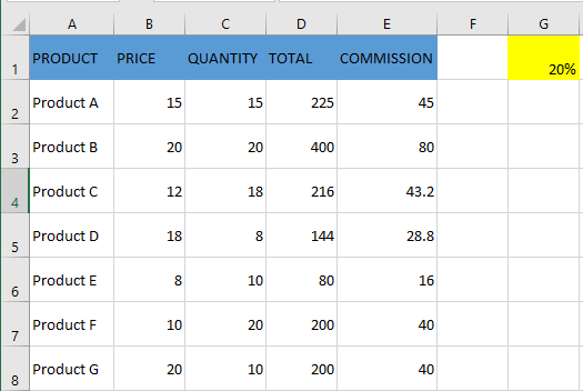
Notice that there are two dollar signs $ in the commission cell reference $G$1. What does the dollar sign do?

A dollar sign, when added before the column letter and row number, makes the reference absolute (i.e., it prevents the row and column from changing when the formula is copied). For example, in the case above, when the formula is copied from E2 to E3, it changes from =D2*$G$1 to =D3*$G$1. Notice that while D2 changes to D3, $G$1 remains the same. This is because both the column G and the row 1 are locked with the $ symbol.

Absolute cell references are useful when you don’t want a reference to change when copying formulas. This is often the case when using a fixed value in a formula (such as a tax rate, commission rate, number of months, etc.).

While you could hardcode this value into the formula (e.g., use 20% instead of $G$1), using a cell reference allows you to update the value later. For example, if the commission rate changes from 20% to 25%, you can simply update the value in cell G1, and all formulas will update automatically.

Mixed Cell References

Mixed cell references are a bit more complex than relative and absolute references. There are two types of mixed references:

• The row is locked while the column changes when the formula is copied.
• The column is locked while the row changes when the formula is copied.

Let’s see how this works with an example.

Below is a dataset where you need to calculate three levels of commission based on the percentage values in cells E2, F2, and G2.

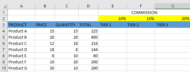
You can now use the power of mixed references to calculate all these commissions with a single formula. Enter the following formula in cell E4 and copy it across all relevant cells:

=$B4*$C4*E$2

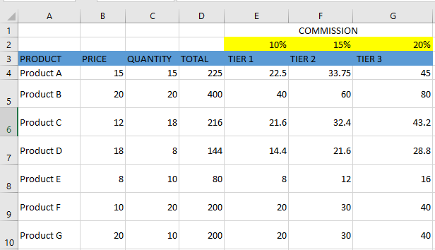
The formula above uses two types of mixed references (one with the row locked, one with the column locked). Let’s analyze each reference:

• $B4 (and $C4) – The dollar sign is placed before the column letter but not before the row number. This means the column is fixed, but the row will adjust when copying the formula down. For example, when copying from E4 to F4, the column stays B and C, but the row changes if you copy downwards.
• E$2 – The dollar sign is placed before the row number but not the column. This means the row is fixed, but the column will adjust when copying the formula horizontally. For example, copying from E4 to F4 changes E$2 to F$2.

How to Change a Reference from Relative to Absolute (or Mixed)

To change a reference from relative to absolute, add a dollar sign before both the column letter and the row number. For example, A1 (relative) becomes $A$1 (absolute).

If you only have a few references to change, you can manually edit them in the formula bar or by selecting the cell and pressing F2.

However, a faster way is to use the F4 keyboard shortcut. When a cell reference is selected (either in the formula bar or in edit mode), pressing F4 toggles the reference type:

• Press F4 once → A1 becomes $A$1 (absolute)
• Press F4 twice → A1 becomes A$1 (row locked)
• Press F4 three times → A1 becomes $A1 (column locked)
• Press F4 four times → reference returns to A1 (relative)