An Excel table is a powerful tool for organizing, analyzing, and managing data efficiently. A typical table consists of three main structural components: the header row, the data body range, and the total row. In addition, Excel tables offer advanced features such as calculated columns and a resizing handle. Below is a detailed explanation of each of these elements.
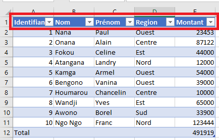
The Header Row
The header row is the topmost row of an Excel table and is typically visible by default. It defines the field names or column headers of your dataset. These headers must be static values (not formulas) to maintain formula references and enable structured references, a key feature in Excel table formulas.
Headers serve two main purposes:
-
They define the identity of each column.
-
They display filter drop-down buttons that provide powerful options to sort and filter data.
Each header value within a single table must be unique. If you accidentally enter duplicate header names, Excel will automatically append a number to one of them to preserve uniqueness (e.g., entering a second “ID” column will result in “ID2”).
To make headers dynamic, you can use data validation lists, allowing users to choose from a predefined list of possible header names. If a header is changed, all formulas referring to that column automatically update accordingly.
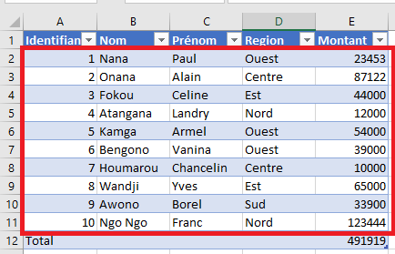
The Data Body Range
This is the central portion of the table, found between the header and the total row. It contains the actual data records. If no data is present, Excel shows a single empty row where data can be entered.
The size of the data body range is only limited by the total number of rows available in the worksheet. The body range grows automatically as you add new entries and is designed to support Excel features like structured referencing, dynamic filtering, and formatting.
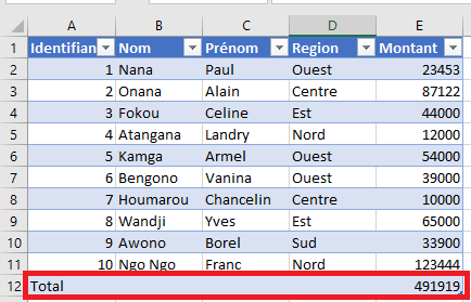
The Total Row
The total row appears at the bottom of the table and is optional. It is hidden by default but can be displayed to provide summary calculations like Sum, Average, Count, Max, Min, etc.
When you select a cell in the total row, a drop-down list appears allowing you to choose a built-in aggregate function. These calculations are automatically adjusted to consider only visible rows, which is useful when filters are applied. You may also insert your own custom formulas, referencing cells inside or outside the table.
Calculated Columns
A calculated column automatically applies the same formula to all cells in that column’s data range. When you enter a formula into a single cell of a calculated column, Excel automatically propagates it throughout the column, maintaining consistency.
If the column contains a mix of values and formulas, and is not yet recognized as a calculated column, Excel will display an AutoCorrect Options button after formula entry. You can use it to convert the column into a fully calculated one.
Note: There is no built-in indicator to show if a column is truly a calculated column. The best method is to edit a formula and observe whether Excel offers to apply it to the entire column.
The Resize Handle
In the bottom-right corner of the table is a small resize handle, a square icon used to adjust the size of the table. By clicking and dragging this handle, you can expand or shrink the table’s range.
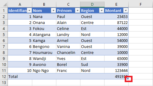
This is useful when adding or removing rows/columns manually. You can also resize the table from the Table Design tab on the ribbon, using the Resize Table option.
Table Behavior and Constraints
Excel imposes several design limitations on tables to preserve functionality:
-
Headers must occupy a single row only.
-
The table can have only one total row.
-
Duplicate column headers are not allowed.
-
Multi-cell array formulas are not permitted (single-cell arrays are allowed).
-
Tables cannot overlap with other tables.
-
Each table must have a unique name within the workbook.
Additionally, you cannot save a workbook with tables in shared mode, although you may publish it via SharePoint for collaborative work.
These rules ensure that Excel can manage structured references, auto-expansion, and dynamic formulas reliably within tables.
Freezing Table Rows
In large tables, identifying columns can become difficult when scrolling down, as the header row disappears from view. To solve this, you can freeze the top row via the ribbon (View > Freeze Panes > Freeze Top Row), ensuring the headers stay visible as you scroll.
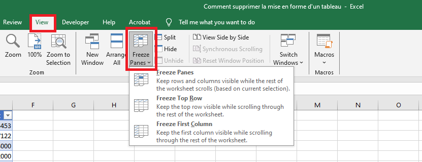
When headers aren’t frozen, Excel compensates by temporarily displaying the table’s headers in place of the usual column letters (A, B, C, etc.) when you’re working inside the table.
Accessibility
Excel supports alternative text (alt text) for tables, helping users who rely on screen readers and other assistive technologies.
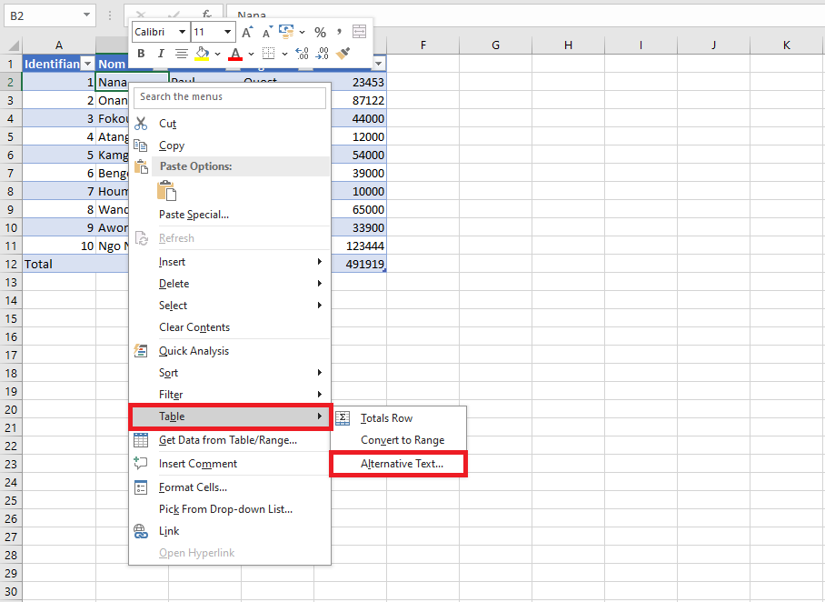 T
T
To set alt text, right-click on any table cell, go to Table > Alt Text, and fill in the description. This improves accessibility for both web publications and documents exported in formats like DAISY. When users hover over a table with alt text, the description appears as a tooltip.