
ANOVA (Analysis of Variance) is a collection of statistical models and procedures used to assess whether there are any statistically significant differences between the means of two or more independent groups. It works by partitioning the observed variance into components attributable to different sources—systematic factors (which are controlled or known influences) and random factors (which arise from natural variability). This helps in evaluating the influence of an independent variable on a dependent variable.
In practical applications, ANOVA is a powerful statistical test available in Excel that enables users to compare the variances among multiple datasets. For instance, when deciding between various alternatives—such as selecting the best product among several options—ANOVA helps identify which option differs significantly from the rest based on quantitative data. By applying ANOVA in Excel, users can conduct comparative analysis across different groups to determine which dataset stands out as statistically superior.
Furthermore, ANOVA is particularly useful in fields like finance and economics. It can be applied to assess how different factors influence stock price fluctuations or market trends. Analysts, economists, and statisticians often use ANOVA to conduct in-depth studies on the stability and performance of financial indices under various market conditions. Additionally, the ANOVA test helps determine whether the results of an experiment are statistically significant or merely due to chance, thereby enhancing the reliability of conclusions drawn from empirical research.
Data Requirements for ANOVA
Before applying an ANOVA test, it is essential to ensure that your data meets the following assumptions and requirements. These conditions help validate the accuracy and reliability of the results obtained through the analysis:
-
Normality:
The data samples must be drawn from populations that follow a normal distribution. This means the distribution of the dependent variable within each group should be approximately bell-shaped and symmetric. -
Random and Independent Sampling:
The data samples must be randomly selected, and each observation in a group should be independent of observations in other groups. In other words, the behavior or outcome of one subject should not influence or depend on another. This ensures that the groups being compared are statistically unrelated. -
Continuous Dependent Variable:
The dependent variable (the outcome being measured) must be quantitative and continuous, such as height, weight, sales amount, or time, rather than categorical or ordinal. -
Homogeneity of Variances (Equal Variance):
The variances of the data across all groups should be approximately equal. This is also known as homoscedasticity, and it ensures that the spread or dispersion of the values is similar across the different groups being compared. -
Independent Variable with Three or More Levels:
The independent variable (the factor being tested) must have three or more categories or groups (e.g., three different teaching methods, treatment types, or regions). ANOVA is specifically designed to compare multiple group means simultaneously.
Types of ANOVA Tests
There are three main types of ANOVA (Analysis of Variance) tests, each designed for specific experimental scenarios depending on the number of independent variables and the structure of the data:
One-Way ANOVA (Single-Factor ANOVA)
One-way ANOVA is used when there is one independent variable with two or more levels (groups) and one continuous dependent variable. This method allows for the comparison of the means of independent groups to determine whether there is a statistically significant difference among them.
-
It is commonly referred to as single-factor ANOVA, as it focuses on the effect of only one factor (independent variable) on the dependent variable.
-
The test is structurally similar to the t-test, but it generalizes the comparison to more than two groups.
-
It assumes that all groups are independent and that data is normally distributed with equal variances.
Example use case: Comparing the average test scores of students from three different schools.
Two-Way ANOVA (Factorial ANOVA)
Two-way ANOVA is used when there are two independent variables. It allows researchers to evaluate:
-
The individual effect of each independent variable on the dependent variable (main effects),
-
And the interaction effect between the two independent variables.
There are two subtypes of Two-Way ANOVA:
- Two-Way ANOVA with Replication:
Used when there are multiple observations for each combination of the independent variable levels. This occurs when different groups are tested under different conditions.
Example: Comparing student performance across three teaching methods and two school types (public/private), with multiple students per group. -
Two-Way ANOVA without Replication:
Applied when there is only one observation for each combination of the factors. Typically used when the same subjects are tested under two different conditions (repeated measures).
Example: Measuring heart rate of the same athlete before and after a training session.
Prerequisites:
-
Both independent variables must be categorical.
-
The dependent variable must be continuous.
-
Observations must be independent, normally distributed, and have equal variances.
N-Way ANOVA / MANOVA (Multivariate ANOVA)
N-Way ANOVA (or Multifactor ANOVA) involves more than two independent variables, each with multiple levels. It is an extension of Two-Way ANOVA and is used to analyze the combined effect of several independent variables on a single dependent variable.
When the analysis involves multiple dependent variables, the method becomes a Multivariate Analysis of Variance (MANOVA). MANOVA is more powerful and provides a broader understanding of how multiple outcomes are affected by one or more independent variables.
-
N-Way ANOVA evaluates the effects of multiple factors on one dependent variable.
-
MANOVA evaluates the effects of multiple factors on two or more dependent variables simultaneously.
Example:
-
N-Way ANOVA: Evaluating how teaching method, school type, and gender affect exam scores.
-
MANOVA: Evaluating how diet and exercise affect both blood pressure and cholesterol levels.
One-Way ANOVA Formula
The one-way ANOVA (Analysis of Variance) is a statistical method used to compare the means of three or more independent groups to determine whether there are statistically significant differences among them. The method is based on analyzing the ratio of variances, using the F-distribution.
In essence, ANOVA compares:
-
The variance between groups (how much the group means deviate from the overall mean)
-
To the variance within groups (how much the individual values within each group deviate from their respective group mean)
F-Ratio (F-Statistic) Formula:
F=MSB/MSEF
Where:
-
F = ANOVA F-statistic (also called the F-ratio)
-
MSB = Mean Square Between groups (variance between group means)
-
MSE = Mean Square Error (variance within the groups)
How MSB and MSE Are Calculated:
-
Mean Square Between (MSB):
MSB=SSB/(k−1)
Where SSB is the Sum of Squares Between groups, and k is the number of groups.
-
Mean Square Error (MSE):
MSE=SSE/(N−k)
Where SSE is the Sum of Squares Within groups, N is the total number of observations, and k is the number of groups.
Degrees of Freedom:
-
df1 (Between Groups) = k−1
-
df2 (Within Groups or Error) = N−k
-
df3 (Total Degrees of Freedom) = N−1
Hypothesis Testing in ANOVA:
-
Null Hypothesis (H₀): All population means are equal
-
Alternative Hypothesis (H₁): At least one population mean is different from the others
Interpreting the F-Statistic:
-
If the calculated F-value is close to 1, it suggests that the variances between the group means and within the groups are similar, indicating no significant difference between the group means — thus, the null hypothesis is likely true.
-
If the F-value is significantly greater than 1, it implies that the group means differ more than would be expected by chance, and the null hypothesis may be rejected.
To make a statistical decision:
-
Compare the calculated F-statistic with the critical F-value from the F-distribution table (based on df1 and df2 at a chosen significance level, usually α = 0.05).
-
If:
Fcalculated>Fcritical
then the result is statistically significant, and we reject the null hypothesis in favor of the alternative.
Example Dataset – Vertical Jump Test
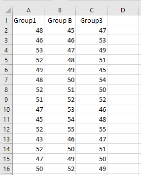
In this example, we have data collected from three different groups of male participants, each group representing a distinct training or demographic category. The data reflects the participants’ performance in a vertical jump test, where the outcome variable is the height jumped, measured in centimeters (cm).
Each column in the dataset corresponds to a different group, and each cell within a column represents the vertical jump height achieved by an individual participant from that group.
This format of data is suitable for conducting a One-Way ANOVA, as it allows us to compare the mean jump heights across the three independent groups to determine whether the differences in performance are statistically significant.
As you can see, each of the three groups consists of 15 participants, resulting in a balanced dataset with a total of 45 observations. The goal is to perform a One-Way ANOVA to determine whether there is a statistically significant difference in the mean vertical jump heights among the three groups.
Steps to Perform One-Way ANOVA in Excel:
To conduct the analysis using Microsoft Excel, follow these steps:
Step 1: Click on “Data Analysis” under the Data tab
To begin, go to the Data tab in the Excel ribbon.
On the far-right side, click on Data Analysis.
This opens the Analysis ToolPak, which contains various statistical tools.
Note: If the “Data Analysis” option does not appear, you need to activate it.
Go to: File → Options → Add-ins → In the Manage box, choose “Excel Add-ins” and click Go → Check Analysis ToolPak → Click OK.

Step 2: Select “Anova: Single Factor”
In the Data Analysis window:
-
Select the first option in the list: Anova: Single Factor.
-
Click OK to proceed.
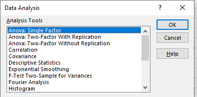
This option is used to test whether there are any statistically significant differences between the means of three or more independent groups.
Step 3: Set Up the ANOVA Parameters
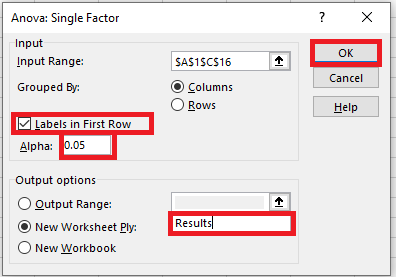
In the Anova: Single Factor dialog box, you need to configure the input settings.
-
Input Range: Select the entire range of your dataset, including all group columns.
You can include the labels in the first row (e.g., Group A, Group B, Group C) if you check the box labeled “Labels in First Row.” -
Grouped By: Choose Columns if your groups are arranged in columns (as in most datasets for ANOVA).
This step defines which data Excel will analyze.
Step 4: Choose How Data Is Grouped
Next, specify whether your data is grouped by columns or rows.
-
In this example, select Columns because each group’s data is arranged in a separate column.
-
If your data were arranged in rows instead, you would select Rows.
Step 5: Indicate if Your Data Includes Labels
If you included the group names or labels in the first row of your selection during the Input Range step, make sure to check the box labeled “Labels in First Row”. This helps Excel correctly identify the groups in the output.
Step 6: Set the Significance Level (Alpha)
The Alpha level represents your threshold for statistical significance.
-
The most commonly used alpha value is 0.05.
-
This means that if the P-value obtained from the ANOVA test is less than or equal to 0.05, you reject the null hypothesis and accept that there is a significant difference between group means.
For this example, leave the alpha level set at 0.05.
Step 7: Choose the Output Location
You have three options for where to place the ANOVA results:
-
Output Range: Select a specific range within your current worksheet where the results will be displayed.
-
New Worksheet Ply: Place the results in a new worksheet within the current workbook. You can name this new sheet (e.g., “Results”).
-
New Workbook: Output the results to an entirely new Excel file.
For this example, select New Worksheet Ply and name the new sheet “Results”.
Step 8: Run the One-Way ANOVA
Finally, click OK to execute the one-way ANOVA test in Excel.
Interpreting the Results
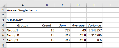
Once Excel completes the analysis, it will generate an ANOVA summary table containing several key statistics. The next step is to interpret these results to determine whether there is a statistically significant difference among the group means.
Detailed ANOVA Report
Summary Table Explained
Here you will find the following key statistics for each group:
-
Sample Size – The number of data points (observations) within each group.
-
Sum – The total sum of all data points in the group.
-
Mean – The average value of the data points in the group.
-
Variance – The average of the squared differences from the mean; it measures the dispersion or spread of values within the dataset.
Analysis of Variance
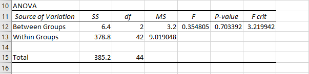
Below is an overview of the ANOVA summary table generated by Excel, which displays the results of the variance analysis.
Understanding the ANOVA Results Table
The results table is divided into three main rows:
-
Between Groups – This row summarizes the variation attributed to differences between the groups.
-
Within Groups (Error) – This row summarizes the variation within each group, often referred to as residual or error variance.
-
Total – This row shows the combined total of the sum of squares and degrees of freedom from the two rows above.
Each column in the table corresponds to a specific statistical measure:
-
Sum of Squares (SS):
Measures the total variation attributed either between groups or within groups. -
Degrees of Freedom (df):
For between groups, calculated as the number of groups minus one (e.g., 3 – 1 = 2).
For within groups, calculated as the total number of observations minus the number of groups (e.g., 45 – 3 = 42). -
Mean Squares (MS):
The average variation calculated by dividing the sum of squares by the corresponding degrees of freedom (MS = SS / df). -
F Statistic (F):
The test statistic used in one-way ANOVA, calculated as the ratio of MS between groups to MS within groups. -
P-Value:
The probability value that indicates the significance level of the test result. -
Critical F (F crit):
The threshold value obtained from the F-distribution table based on the degrees of freedom and the chosen significance level (alpha).
Hypotheses for One-Way ANOVA
-
Null Hypothesis (H₀):
There is no difference between the mean values of the three groups. -
Alternative Hypothesis (H₁):
At least one group mean is different from the others.
Interpreting the P-Value
Recall that earlier you specified an alpha level of 0.05.
-
If the P-value ≤ 0.05, you reject the null hypothesis, indicating a statistically significant difference between the group means.
-
If the P-value > 0.05, you fail to reject the null hypothesis, indicating that there is no statistically significant difference between the group means.
In this example, since the P-value is greater than 0.05, we do not reject the null hypothesis. This means there is no evidence of a difference in the average vertical jump heights among the three groups. In other words, all groups performed approximately the same on the vertical jump test.
Post-Hoc Tests
If the one-way ANOVA result is significant (i.e., P ≤ α), the ANOVA tells you that there is a difference somewhere among the group means but does not specify where the difference lies.
To pinpoint which specific groups differ from each other, you need to perform post-hoc tests such as:
-
Tukey’s HSD (Honestly Significant Difference)
-
Bonferroni correction
-
Scheffé’s test
These tests help compare each pair of group means to identify the exact pairs with statistically significant differences.
What is ANCOVA?
ANCOVA stands for Analysis of Covariance. It can be understood as an extension of the ANOVA test. ANCOVA combines elements of ANOVA and regression analysis. For example, if all independent variables act as covariates, ANCOVA essentially becomes a regression analysis; thus, it is a hybrid between ANOVA and regression.
This method accounts for and controls the effects of covariates, improving the accuracy of an experiment. Covariates are characteristics of the participants that are not the focus of the study but can potentially influence the dependent variable (outcome).
Example: ANOVA vs. ANCOVA
Imagine a study investigating the effects of a specific medication on a disease in participants of varying ages.
-
The independent categorical variable (factor) is the treatment group (medication vs. placebo).
-
The continuous covariate is age.
-
The dependent variable is the change in disease status after treatment.
-
Here, ANCOVA would be used because it controls for age as a covariate while assessing the treatment effect.
-
By contrast, ANOVA would be used if age is not considered a continuous independent variable and the analysis focuses only on the treatment groups and their effect on disease progression.
Statistical Methods: ANOVA, ANCOVA, MANOVA, and Regression
-
MANOVA (Multivariate ANOVA) is similar to ANOVA but involves multiple continuous dependent variables instead of just one.
-
In regression analysis, the predictors can be continuous variables, whereas ANOVA typically uses categorical predictors.
Comparison Table: ANOVA vs. ANCOVA
| Aspect | ANOVA | ANCOVA |
|---|---|---|
| Definition | Analysis of variance | Analysis of covariance |
| Purpose | Tests variance or differences between means of 3+ groups | Evaluates the mean of a dependent variable based on a categorical independent variable while controlling for covariates |
| Model Type | Can involve linear and non-linear models | Uses only linear models |
| Independent Variables | Categorical | Both categorical and continuous (covariates) |
| Covariate Treatment | Ignores covariate influence | Accounts for and controls the effects of covariates |
Key Differences Between Regression and ANOVA
-
Regression mainly applies to fixed or independent variables; ANOVA applies to random variables.
-
Regression can be linear or multiple regression, whereas ANOVA has popular types such as random effects, fixed effects, and mixed effects models.
-
Regression is used for estimating or predicting a dependent variable from one or more independent variables. ANOVA is used to find a common mean among groups.
-
Regression typically has one error term, while ANOVA has more than one error term.
Comparison Table: Regression vs. ANOVA
| Aspect | Regression | ANOVA |
|---|---|---|
| Definition | Statistical method to model relationships between variables | Analysis of variance, used to determine if unrelated groups have a common mean |
| Variable Nature | Applied to fixed or independent variables | Applied to random variables |
| Types | Mainly linear and multiple regression | Random effects, fixed effects, and mixed effects ANOVA |
| Examples | Predicting raw material prices based on Brent crude price | Comparing results from different research teams on unrelated products |
| Variables Used | One dependent and one or more independent variables | Different variables that are not necessarily related |
| Purpose | Used for prediction and estimation | Used to test differences between group means |
| Error Terms | Typically one residual (error) term | More than one error term |
Regression and ANOVA are both powerful statistical tools applied to multiple variables:
-
Regression is used for predicting the dependent variable based on one or more independent variables, usually fixed or continuous.
-
ANOVA is used to compare means across groups that are unrelated, focusing on identifying whether group means differ significantly rather than prediction.
ANCOVA extends ANOVA by controlling for continuous covariates, allowing for more precise interpretation when confounding variables may affect the dependent variable.