All cell contents initially use the same default formatting, which can make it difficult to read a workbook with a lot of information. Basic formatting helps personalize the appearance of your workbook, allowing you to draw attention to specific sections and make your content easier to read and understand.
You can also apply number formatting to tell Excel exactly what type of data you’re using in your workbook, such as percentages (%), currency ($), and more.
Changing the Font
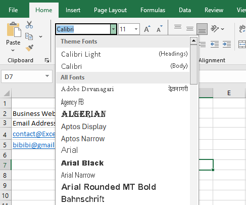
By default, the font in every new workbook is set to Calibri. However, Excel offers many other fonts to help you customize the text in your cells.
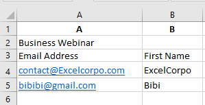
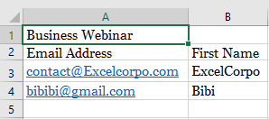
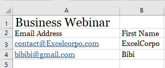
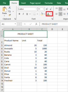
In the example below, we’ll format the title cell to distinguish it from the rest of the worksheet.
- Select the cell(s) you want to modify.
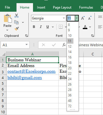
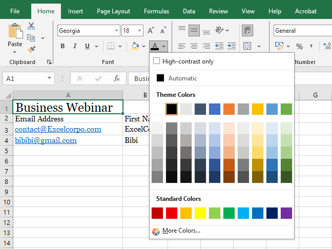
- Click the drop-down arrow next to the Font command on the Home tab.
The font menu will appear. - Select the desired font. A live preview will appear as you hover over different options.
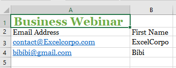
In our example, we’ll choose Georgia.
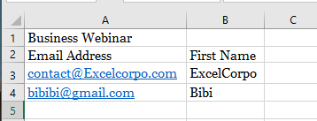
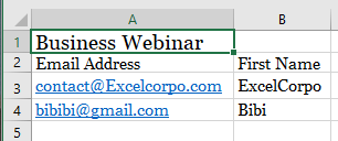
- The text will update to the selected font.
For professional workbooks, choose an easy-to-read font. Besides Calibri, good options include Cambria, Times New Roman, and Arial.
Changing the Font Size
- Select the cell(s) you want to modify.
- Click the drop-down arrow next to the Font Size command on the Home tab.
The font size menu will appear. - Select the desired font size. A live preview will appear as you hover.
In our example, we’ll choose 16 to enlarge the text.
- The text will update to the selected size.
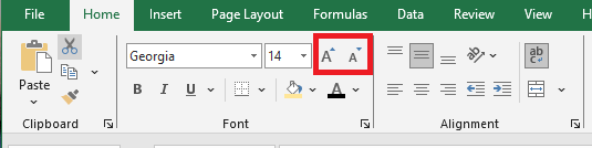
You can also use the Increase Font Size and Decrease Font Size buttons or type a custom size using your keyboard.
Changing the Font Color
In Excel, you can add visual interest by changing the font color. While spreadsheets are often used to display specific data, that doesn’t mean they have to look plain. Adding a touch of color can make your sheets more appealing and easier to read.
You can choose a theme color, a standard Excel palette color, or create a custom one.
- Select the cell(s) you want to modify.
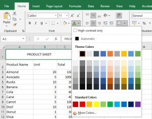
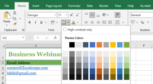
- Click the drop-down arrow next to the Font Color command on the Home tab.
The color menu will appear. - Select the desired color. A live preview appears as you hover.
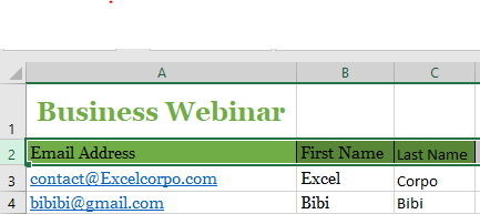
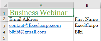
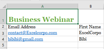
In our example, we’ll choose Green.
- The text will update to the selected color.
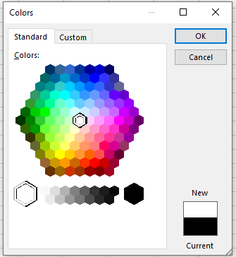
To access more color options, click More Colors at the bottom of the menu.
Adding a Background Color to a Cell Range
You can make a range stand out by applying a background color.
If you want to change the background color based on cell values (e.g., red for negative, green for positive), conditional formatting is more suitable.
You can use a theme color, a standard color, or a custom one.
- Select the range you want to format.
- Click the Home tab.
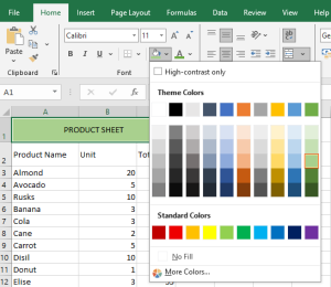
- Click the Fill Color drop-down list.
- Click a theme color or a standard color.
Excel applies the fill color to the selected range.
To remove the background color, select No Fill.
To use a custom color:
- Select the range.
- Go to Home > Fill Color > More Colors.
- Choose a color or click the Custom tab to adjust RGB values.
- Click OK.
Using Bold, Italic, and Underline Commands
To enhance appearance and impact, apply text effects like:
- Bold: to highlight labels
- Italic: to emphasize text
- Underline: for titles and headers
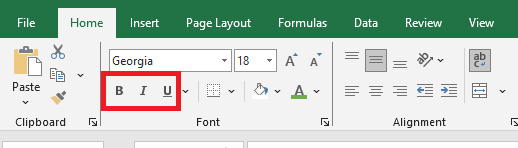
- Select the cell(s) you want to modify.

- Click the Bold (B), Italic (I), or Underline (U) button on the Home tab.
In our example, we’ll bold the selected cells.
- The selected effect will apply to the text.
You can also use keyboard shortcuts:
- Ctrl+B = Bold
- Ctrl+I = Italic
- Ctrl+U = Underline
Text Alignment
By default:
- Text is bottom-left aligned
- Numbers are bottom-right aligned
You can change alignment to improve readability.
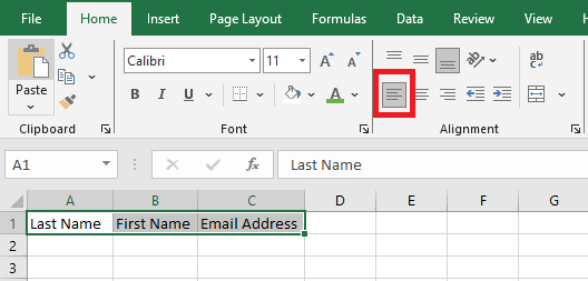
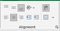
Horizontal alignment:
- Left Align: aligns content to the cell’s left edge
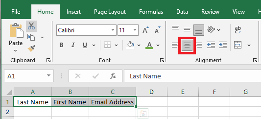
- Center Align: centers content horizontally
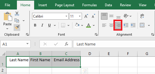
- Right Align: aligns content to the right
Vertical alignment:
- Top Align: aligns content to the top
- Middle Align: centers content vertically
- Bottom Align: aligns content to the bottom
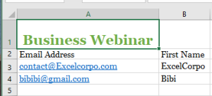
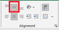
To apply horizontal alignment:
- Select the cell(s).
- On the Home tab, click one of the three horizontal alignment buttons.
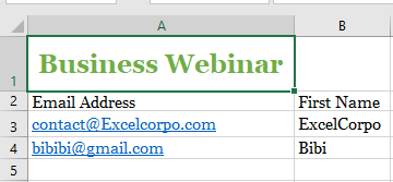
In our example, we select Center Align.
- The text realigns accordingly.
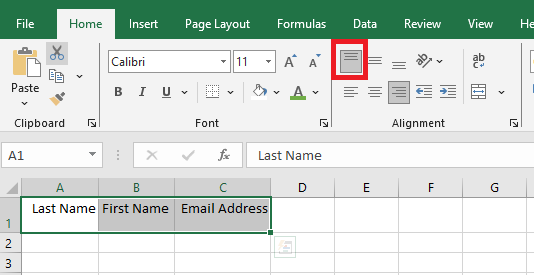
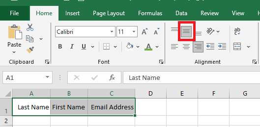
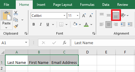
To apply vertical alignment:
- Select the cell(s).
- Choose one of the three vertical alignment options.
In our example, we choose Middle Align.
- The text is realigned.
You can combine both vertical and horizontal alignment.
Cell Borders and Fill Colors
Cell borders and fill colors help define clear boundaries in your spreadsheet. Below, we’ll apply both to header cells.
To add a border:
- Select the cell(s).

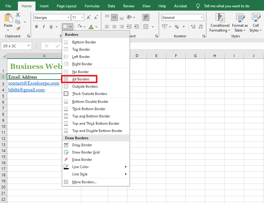
- Click the Borders drop-down arrow on the Home tab.
The border menu appears. - Select a border style (e.g., All Borders).
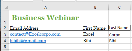
- The selected border appears.
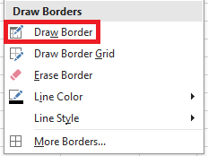
To customize line style and color, use the Draw Borders tools at the bottom of the menu.
To add a fill color:
- Select the cell(s).
- Click the Fill Color drop-down on the Home tab.
- Choose a color. Live preview is available.
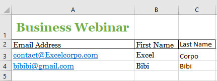
In our example, we select Light Green.
The fill color is applied.