When you enter a number in a cell, you can display that number in a variety of different formats. Excel has quite a few built-in number formats, but sometimes none of them are exactly what you need. This chapter explains how to create custom number formats and provides many examples that you can use as-is or adapt to your needs.
About Number Format
By default, all cells use the General number format (what you type is what you get). But if the cell is not wide enough to display the entire number, the General format rounds decimal numbers and uses scientific notation for large numbers. In many cases, the General number format works just fine, but most people prefer to specify a different number format for better consistency.
Excel automatically applies a built-in number format to a cell based on the following criteria:
■ If a number contains a slash (/), it may be converted to a date or fraction format.
■ If a number contains a dash (-), it may be converted to a date format.
■ If a number contains a colon (:) or is followed by a space and the letter A or P (uppercase or lowercase), it may be converted to a time format.
■ If a number contains the letter E (uppercase or lowercase), it may be converted to scientific notation (also called exponential format). If the number doesn’t fit the column width, it may also be converted to this format.
Formatting Numbers Using the Ribbon
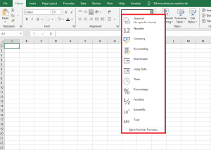
The Number group on the Home tab of the Ribbon contains several commands for quickly applying common number formats. The Number Format drop-down menu gives you quick access to 11 common number formats.
Additionally, the Number group contains a few buttons. When you click one of these buttons, the selected cells adopt the specified number format. The table below summarizes the formats these buttons apply.
| Shortcut | Applied Formatting |
|---|---|
| Ctrl+Shift+~ | General format (unformatted values) |
| Ctrl+Shift+$ | Currency format with two decimal places (negative numbers appear in parentheses) |
| Ctrl+Shift+% | Percentage format with no decimals |
| Ctrl+Shift+^ | Scientific notation format with two decimal places |
| Ctrl+Shift+# | Date format with day, month, and year |
| Ctrl+Shift+@ | Time format with hour, minute, and AM/PM |
| Ctrl+Shift+! | Two decimals, thousand separator, dash for negative values |
Using the Format Cells Dialog Box to Format Numbers
For maximum control over number formatting, use the Number tab in the Format Cells dialog box. You can access this dialog box in several ways:
■ Click the dialog box launcher in the lower-right corner of the Number group on the Home tab.
■ Choose Home / Number / Number Format / More Number Formats.
■ Press Ctrl+1.

The Number tab of the Format Cells dialog box contains 12 number format categories to choose from. When you select a category in the list box, the right side of the dialog updates to display the appropriate options.
Here are the number format categories, along with some general comments:
■ General: Default format; displays numbers as integers, decimals, or scientific notation if the value is too wide for the cell.
■ Number: Specify decimal places, whether to use the system’s thousands separator (e.g., a comma), and how to display negative numbers.
■ Currency: Specify decimal places, choose a currency symbol, and display negative numbers. This format always uses the system’s thousands separator.
■ Accounting: Similar to Currency but aligns currency symbols vertically, regardless of the number of digits.
■ Date: Choose from a variety of date formats and select regional settings for date formatting.
■ Time: Choose from a variety of time formats and select regional settings for time formatting.
■ Percentage: Choose the number of decimals; always displays a percent sign.
■ Fraction: Choose from nine fraction formats.
■ Scientific: Displays numbers in exponential notation (with an E): e.g., 2.00E+05 = 200,000. You can choose the number of decimal places to show before the E.
■ Text: When applied, Excel treats the value as text (even if it looks like a number). Useful for things like numeric part numbers or credit card numbers.
■ Special: Contains additional formats. The list varies based on the selected locale. For U.S. English, formatting options include ZIP Code, ZIP+4, phone number, and Social Security number.
■ Custom: Define number formats not included in the other categories.
NOTE
If a cell displays a series of hash marks (such as #########) after you apply a number format, this usually means the column is not wide enough to display the value using the selected format. Widen the column (by dragging the right border of the column header) or change the number format. A series of hash marks can also mean the cell contains an invalid date or time.
Creating a Custom Number Format
When you create a custom number format, it can be used to format any cell in the workbook.
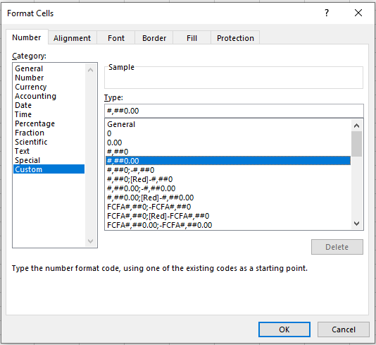
You can create about 200 custom number formats per workbook. The following figure shows the Custom category in the Number tab of the Format Cells dialog box.
You can create number formats not included in the other categories. Excel gives you great flexibility in defining custom number formats.
Custom number formats are stored in the workbook in which they are defined. To make a custom format available in another workbook, simply copy a cell using the custom format to the other workbook.
Parts of a Numeric Format String
Number format codes are strings of symbols that define how Excel displays the data stored in cells. We’ll explain how to write formats, but first we need to clarify how Excel interprets these symbols.
Each numeric format code can contain up to four sections, separated by semicolons (;), allowing you to specify different format codes for positive numbers, negative numbers, zero values, and text. The codes follow this order:
Positive Format ; Negative Format ; Zero Format ; Text Format
If you don’t use all four sections in a format string, Excel interprets it as follows:
■ If you use only one section: it applies to all numeric values.
■ If you use two sections: the first applies to positive values and zeros, the second to negative values.
■ If you use three sections: the first applies to positives, the second to negatives, and the third to zeros.
■ If you use all four sections: the last applies to text stored in the cell.
You can choose to skip formatting for any section by entering General. For example, if you only want to format positive numbers and text, you could use a format string like:
Section1; General; General; Section4
Note that General removes any special formatting from the data entered—so be careful. Negative numbers using General will not display a minus sign.
Custom Number Format Codes
The table below lists formatting codes for custom formats, along with brief descriptions.
| Code | Description |
|---|---|
| General | Displays the number in General format. |
| # | Placeholder for optional digits. If not needed, the digit is not shown. Used for more readable numbers. |
| 0 | Placeholder for mandatory digits. Even if a digit is not significant, it will display. Example: 0.00 always shows two decimals. |
| , (comma) | Indicates the location of the decimal or thousands separator. |
| % | Percentage format. |
| (space) | Thousand separator placeholder. Helps define behavior for thousands/millions. |
| E-, E+, e-, e+ | Scientific notation. |
| \ | Displays the character following the backslash as-is. |
| ? | Placeholder that aligns decimals by spacing insignificant zeros. Useful in fractions. |
| * | Repetition modifier. Used with a character to fill the cell with that character. |
| _ (underscore) | Space modifier. Inserts a space equal to the width of the specified character. Useful for aligning parentheses. |
| « text » | Displays the text within double quotes. |
| @ | Text placeholder. |
| [Color] | Displays characters in a specified color. |
| [Color n] | Displays the corresponding color from the palette (n = 0 to 56). |
| [Condition] | Sets your own condition for each section of a number format. |
Example 1: Changing Font Color
One of the simplest things you can do with number format codes is change the font color. The syntax is: [ColorName]
For example, you can assign a different color for each section of the format string:
[Red]General;[Blue]General;[Magenta]General;[Cyan]General
This results in:

Note that the negative number in line 3 no longer displays a minus sign. Also, color formatting does not affect decimal places or text alignment.
Example 2: Adding Text with Format Codes
You can add text to numbers using format codes in two ways:
Single characters: To prefix a symbol like @, type a backslash (\) followed by the symbol.
Example:
\@General
Results in output:
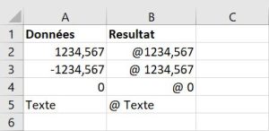
Full text strings: To append text like « units », enclose the string in double quotes:
Example:
General" units"
Results in output:

If extended to all four sections like this:
General" units"; General" units"; General" units"; General" units"
Then the output looks like:
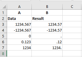
Example 3: Zero (0)
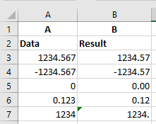
Here is an example using the zero placeholder. The following format:
0.00
Ensures that numbers always display with two decimal places, even if the decimal part is zero.
Merci pour la suite du texte. Je vais maintenant te fournir la traduction complète en anglais de cette nouvelle section, en conservant le style technique du guide Excel.
Zeros in a number format code represent mandatory digits.
Example 4: Question Mark (?)
Here is an example of the question mark code in action. The following format code is used:
0,??

A question mark is a placeholder for a digit. It adds space for insignificant zeros on either side of the decimal point so that decimals align properly when using a fixed-width font.
Example 5: Hash Symbol (#)
Here is an example of the hash symbol code in action. The following format code is used:
#, ##
The hash symbol represents an optional digit. If the digit is not needed, it will not be displayed in the formatted number.
Example 6: Space
Here is an example of the space code in action. The following format is used:
$??? ???,00

The space character in number format codes acts as a placeholder for thousands separators.
Example 7: Asterisk (*)
Here is an example of the asterisk code in action. The following format is used:
*=0.##

The asterisk is a repeating character modifier. It repeats the character to fill the remaining width of the cell.
Example 8: Underscore (_)
Here is an example using the underscore code. Format used:
_(#,##_);(#,##)

The underscore creates a blank space equal to the width of the character following it. It is useful for aligning positive and negative numbers, especially when negative values use parentheses.
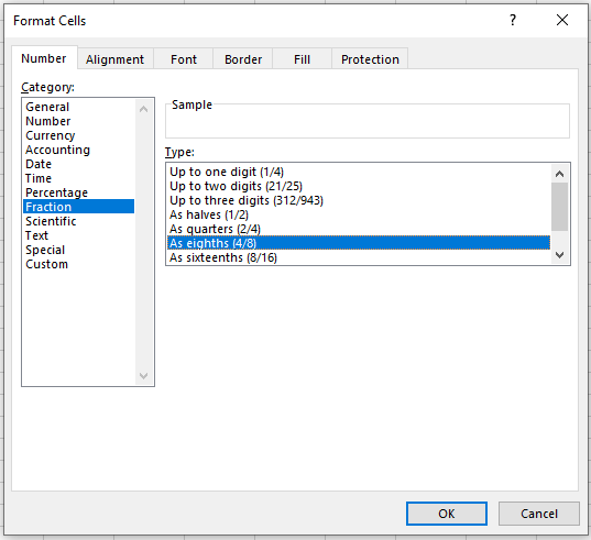
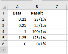
Example 9: Fractions ( / )
Excel supports several built-in fraction formats (found under the « Fraction » category in the Format Cells dialog box). For example, to display 0.125 as an eighth, select As eighths (4/8) from the Type list.
Fractions are special because they involve unit conversion. For example:
- 0.23 is shown as 23/100,
- 0.25 can be simplified to 1/4,
- 1.25 can be shown as 1 1/4 or 5/4.
Excel rounds to the closest fraction based on the format code and follows the same rules as the hash and question mark symbols.
Mixed Fractions (Integer with Reduced Fraction)
A typical format separates the integer part from the fractional part. Use question marks for better alignment:
#???/???

This preserves the alignment of the fraction bar regardless of digit count. For example:
#??/??
Displays 0.23 as 3/13 instead of 23/100.
Improper Fractions
If you prefer to merge the whole number into the fraction:
###/###
This creates an improper fraction format with up to three digits.
Fixed-Base Fractions
To force Excel to round to a fixed denominator, include it in the format code:
###/15
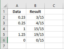
The value is rounded to the nearest 15th.
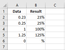
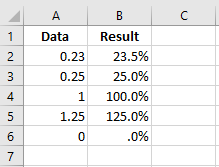
Example 10: Percentages (%)
Like fractions, percentages are controlled by format codes. A simple format might be:
#%
You can also specify fractional percentages:
##/#%
This shows percentages as simplified fractions.
You can also include decimals:
#,0%
Example 11: Scientific Notation (E)
Large or tiny numbers are difficult to read with standard notation. Scientific notation shifts the decimal point for clarity:
- 0.0000001 becomes 1 × 10⁻⁷
- Excel shows this as
1E-07
The capital letter E signals scientific notation.
A format like #E+# shows the base and exponent, while:
0.00E+00
forces both parts to show two digits.


This provides consistent display with predictable string length.
Scaling Values
Custom formats can also scale numbers. For instance, you might want to display numbers in thousands or millions, while preserving the actual value for calculations.
Displaying Thousands
Format: # ### (space at the end)
This removes the last three digits and rounds to the nearest integer.
Format: # ###,00
Rounds to two decimals.
| Value | Format | Display |
|---|---|---|
| 123456 | # ### |
123 |
| 1234565 | # ### |
1,235 |
| -323434 | # ### |
–323 |
| 123123.123 | # ### |
123 |
| 499 | # ### |
1 |
| 123456 | # ###,00 |
123.46 |
| 499 | # ###,00 |
0.50 |
Displaying Hundreds
Format: 0","00
Divides by 100 and displays two decimals.
| Value | Format | Display |
|---|---|---|
| 546 | 0","00 |
5.46 |
| 500 | 0","00 |
5.00 |
| -500 | 0","00 |
–5.00 |
Displaying Millions
Format: # ### (two spaces)
or # ###,00
or # ### "M"
or complex format:
# ###,0 "M"_);(# ###,0 "M)";0,0"M"_
| Value | Format | Display |
|---|---|---|
| 123456789 | # ### |
123 |
| 1.23457E+11 | # ### |
123,457 |
| 5000000 | # ###,00 |
5.00 |
| -5000000 | # ###,00 |
–5.00 |
| 0 | # ###,00 |
0.00 |
| 1000000 | # ### "M" |
1M |
| 0 | # ###,0 "M"_);(# ###,0 "M)";0,0"M"_ |
0.0M |
| –5000000 | same complex format | (5.0M) |
Custom Date and Time Format Codes
| Code | Description |
|---|---|
| m | Month (1–12, no leading zero) |
| mm | Month (01–12) |
| mmm | Abbreviated month (Jan, Feb) |
| mmmm | Full month name |
| d | Day (1–31, no leading zero) |
| dd | Day (01–31) |
| ddd | Abbreviated weekday (Mon, Tue) |
| dddd | Full weekday (Monday, Tuesday) |
| yy | Year (2 digits) |
| yyyy | Year (4 digits) |
| h | Hour (0–23, no leading zero) |
| hh | Hour (00–23) |
| s | Second (0–59) |
| ss | Second (00–59) |
| [ ] | Display times above 24h or minutes >60 |
| AM/PM | 12-hour clock |
| \ | Escapes next character |
| . | Decimal point |
| « text » | Displays quoted text |
Dates entered are formatted based on the system’s short date. This can be adjusted in Windows settings.
| Value | Format | Display |
|---|---|---|
| 42552 | mmmm d, yyyy (dddd) |
July 1, 2016 (Friday) |
| 42552 | "Today is" dddd! |
Today is Friday! |
| 42552 | dddd, mm/dd/yyyy |
Friday, 07/01/2016 |
| 0.345 | h:mm "hours" |
8:16 hours |
| 0.78 | h:mm a/p".m." |
6:43 p.m. |
Conditional Format Specification
The following format displays different text depending on the cell’s value:
[<10]"Too Low";[>10]"Too High";"Just Right"
- If value < 10 → displays “Too Low”
- If value > 10 → displays “Too High”
- If value = 10 → displays “Just Right”
Note: Only one or two conditions are allowed, plus a default fallback.
In most cases, Excel’s built-in Conditional Formatting feature is a better solution for value-based styling.