
The chi-square test is a non-parametric statistical method used to examine the association between two or more categorical variables based on randomly selected data samples. This test helps determine whether there is a significant relationship or dependency between the variables under study.
In Excel, performing a chi-square test involves calculating the p-value, which indicates the probability that any observed differences occurred by chance. Since Excel does not provide a built-in, direct chi-square test function, users rely on mathematical formulas and functions to compute the test statistic and its associated p-value.
There are two main types of chi-square tests commonly used in statistical analysis:
-
Chi-Square Goodness-of-Fit Test:
This test assesses whether the observed frequency distribution of a single categorical variable matches an expected distribution. It answers questions such as: “Does this sample data fit the expected proportions?” -
Chi-Square Test of Independence:
This test evaluates whether two categorical variables are independent of each other or if there is a significant association between them. It is commonly applied to contingency tables to test relationships between variables.
Chi-Square Goodness-of-Fit Test
The goodness-of-fit test is a statistical method used to determine whether the observed sample data correspond to a specific theoretical distribution or population. In other words, it assesses how well the sample data fit a set of expected observations.
The chi-square test statistic is denoted by the symbol χ2\chi^2 (read as « chi-square »). This statistic is calculated as the sum of the squared differences between the observed and expected frequencies, divided by the expected frequencies for each category.
Mathematically, the chi-square goodness-of-fit formula is expressed as:

Where:
-
χ2* is the chi-square test statistic
-
Oi represents the observed frequency
-
Ei represents the expected frequency
-
i is the index of the category, ranging from 1 to
-
is the total number of categories
-
The degrees of freedom (df) for this test is calculated as df=k−1
Applications of the Chi-Square Goodness-of-Fit Test
This test is widely used in various fields to analyze categorical data and check hypotheses about distributions. Some typical applications include:
-
Evaluating the creditworthiness of borrowers by analyzing their age groups and history of debts to see if the observed default rates fit expected patterns.
-
Investigating the relationship between sales performance and the type or amount of training received by sales representatives.
-
Comparing the returns of a single stock against the returns of the overall sector to see if the stock’s performance aligns with sector trends.
-
Assessing the impact of a television advertising campaign on a specific demographic of viewers by comparing observed viewer responses with expected levels.
Chi-Square Test for Independence
The Chi-Square test for independence is a statistical method used to determine whether two categorical variables are independent or related to each other. Two random variables are said to be independent if the probability distribution of one variable is not influenced or affected by the other variable.
Formula of the Chi-Square Test for Independence:
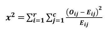
Where:
-
χ2 (chi-square) is the test statistic measuring the difference between observed and expected frequencies.
-
Oij is the observed frequency count in the cell located at the ith row and jt column of the contingency table.
-
Eij is the expected frequency count in the same cell under the assumption that the variables are independent.
-
r is the total number of rows in the contingency table.
-
c is the total number of columns in the contingency table.
-
Degrees of freedom (df) for the test are calculated as:
df=(r−1)(c−1)
Calculation of Expected Frequencies:
The expected frequency EijE_{ij} for each cell in the contingency table is calculated by:

This formula assumes the null hypothesis that the variables are independent, allowing us to estimate what frequency counts would be expected if no association exists.
Interpreting the Chi-Square Test for Independence:
The chi-square statistic (χ2\chi^2) measures how much the observed frequencies deviate from the expected frequencies. Specifically, it quantifies whether the differences between observed and expected counts are larger than what might be reasonably attributed to random chance.
-
A large χ2 value suggests that the observed data differ significantly from what we would expect if the variables were independent, implying a potential association between the variables.
-
A small χ2 value indicates that any observed differences could plausibly be due to random sampling variability, supporting the idea that the variables are independent.
The p-value associated with the test statistic represents the probability that the observed deviations (or more extreme) could occur by chance if the null hypothesis of independence were true. The p-value ranges between 0 and 1:
-
For example, a p-value of 0.0254 indicates there is a 2.54% probability that the observed association is due to chance alone.
-
The smaller the p-value, the stronger the evidence against the null hypothesis.
-
When the p-value is below a predetermined significance level (commonly 0.05), the null hypothesis of independence is rejected, and it is concluded that there is a statistically significant association between the variables.
Applications of the Chi-Square Test for Independence:
This test is particularly useful in the following situations:
-
When there are two categorical variables and the goal is to determine whether an association exists between them.
-
When analyzing contingency tables (cross-tabulations) to examine relationships between multiple categorical variables.
-
When dealing with qualitative data that cannot be quantified directly, such as determining if health plan variations differ across age groups or categories.
Key Characteristics of the Chi-Square Test
The Chi-Square test is a widely used non-parametric statistical method. Its main characteristics can be described as follows:
■ Assesses the Difference Between Observed and Expected Frequencies:
The Chi-Square test is primarily used to evaluate whether the observed frequencies in a dataset significantly deviate from the frequencies that would be expected under a specific null hypothesis. This helps determine if the deviations are due to chance or indicate a statistically significant effect.
■ Tests the Goodness of Fit:
It is employed to assess how well a theoretical distribution fits the observed data. In a goodness-of-fit test, the Chi-Square statistic quantifies the discrepancy between expected and actual data across various categories.
■ Analyzes Relationships Between Categorical Variables:
In contingency tables (also called cross-tabulations), the Chi-Square test is used to analyze the association or independence between two or more categorical variables. It helps answer questions such as whether gender is associated with product preference, or whether a treatment is linked to a certain outcome.
■ Applicable to Nominal Data:
The test is designed for use with categorical variables, particularly those measured at the nominal level (e.g., gender, color, type of product). It does not require interval or ratio data, making it suitable for qualitative analysis.
Perform the Chi-Square Test in Excel
A restaurant manager seeks to examine the relationship between the quality of service and the income level of customers who are waiting to be served.
To conduct this analysis, she follows a structured approach:
-
A random sample of 100 customers is selected to ensure that the results are representative of the overall customer base.
-
Each customer in the sample is asked to evaluate the quality of the service they received using three qualitative categories: “Excellent,” “Good,” and “Poor.”
Based on this setup, the manager formulates the following statistical hypotheses:
-
Null Hypothesis (H₀): There is no association between the quality of service perceived by customers and their income level while waiting to be served.
-
Alternative Hypothesis (H₁): There is an association between the quality of service and the income level of customers waiting to be served.
To further refine the analysis, the manager categorizes customer income levels into three distinct groups:
-
Low income,
-
Middle income, and
-
High income.
She sets the level of significance (α) at 0.05, which means that she is willing to accept a 5% probability of incorrectly rejecting the null hypothesis (Type I error).This setup suggests the use of a Chi-Square Test of Independence to determine whether there is a statistically significant relationship between service quality ratings and income categories.
The results are presented as nine distinct data points, which are systematically outlined in the table below for ease of analysis and interpretation.
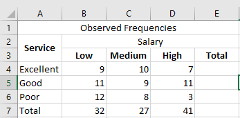
Let us calculate the sum of all the rows and columns. We use the following SUM formula to add the values in the fourth row.
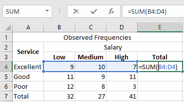
Press the « Enter » key, and the sum appears in cell E4. The output is 26.
Similarly, we apply the SUM formula to the remaining rows and columns. There are 27 respondents with an average salary, and 51 respondents rated the service quality as “Good.”
We apply the formula « (r–1)(c–1) » to calculate the degrees of freedom (df). df = (3–1)(3–1) = 2 × 2 = 4
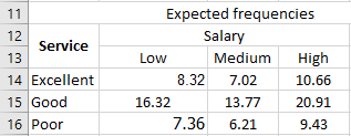
We then use the following formula to calculate the expected frequency for column B and row 4: =B7 * E4 / B9
This calculation is illustrated in the image below.
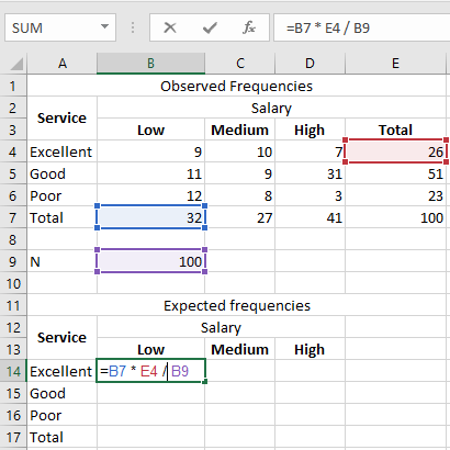
The expected number of customers with a “Low” income who rated the dining service as “Excellent” is 8.32.
In the following calculations, E11 represents the expected frequency for the first row and the first column. E12 corresponds to the first row and the second column.
-
E11 = (26 × 32) / 100 = 8.32
-
E12 = 7.02
-
E13 = 10.66
-
E21 = 16.32
-
E22 = 13.77
-
E23 = 20.91
-
E31 = 7.36
-
E32 = 6.21
-
E33 = 9.43
Similarly, we calculate the expected frequencies for the entire table, as shown in the image below.
Let us calculate the chi-square data points using the following formula:
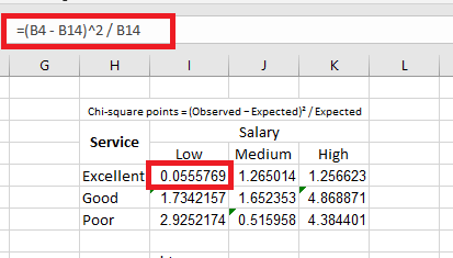
Chi-square points = (Observed − Expected)² / Expected
We apply the formula =(B4 - B14)^2 / B14 to calculate the first chi-square point.
We copy and paste the formula into the remaining cells. This is done to fill in the values across the entire table, as illustrated in the image below.
Let us calculate the chi-square test statistic by summing all the values presented in the following table.
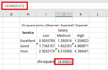
The calculated chi-square value is 18.65823.
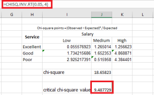
To calculate the critical value, we use either the chi-square critical value table or the formula CHISQ.INV.RT. The formula takes two arguments — the probability and the degrees of freedom.
The probability is 0.05, which represents the significance level. The degrees of freedom (df) is 4.
Let’s find the p-value of the chi-square test using the following formula: =CHISQ.TEST(actual_range, expected_range)
We apply the formula =CHISQ.TEST(B4:D6, B14:D16).
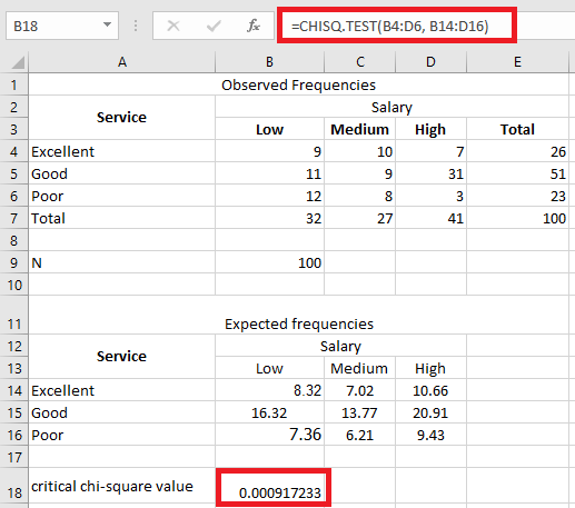
The p-value of the chi-square test is 0.00091723.