When your spreadsheet contains a large amount of data, it can become challenging to quickly locate the information you need. Excel’s filtering feature allows you to refine your data view by displaying only the rows that meet specific criteria. Below is a comprehensive guide to using filters effectively in Excel.
Applying Basic Filters
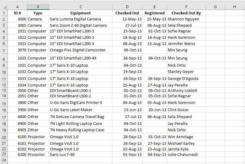
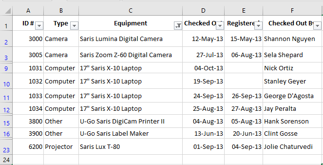
In this section, we’ll apply a filter to an equipment log spreadsheet to display only laptops and projectors that are available for payment.
-
Ensure your spreadsheet has a header row. This row (usually the first) contains labels for each column such as ID#, Type, Equipment, etc. These labels are required for Excel to identify which fields to filter.
-
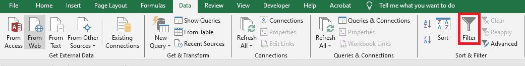
Go to the Data tab and click the Filter command.
-
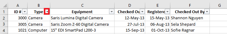
A dropdown arrow will appear next to each header cell.
-
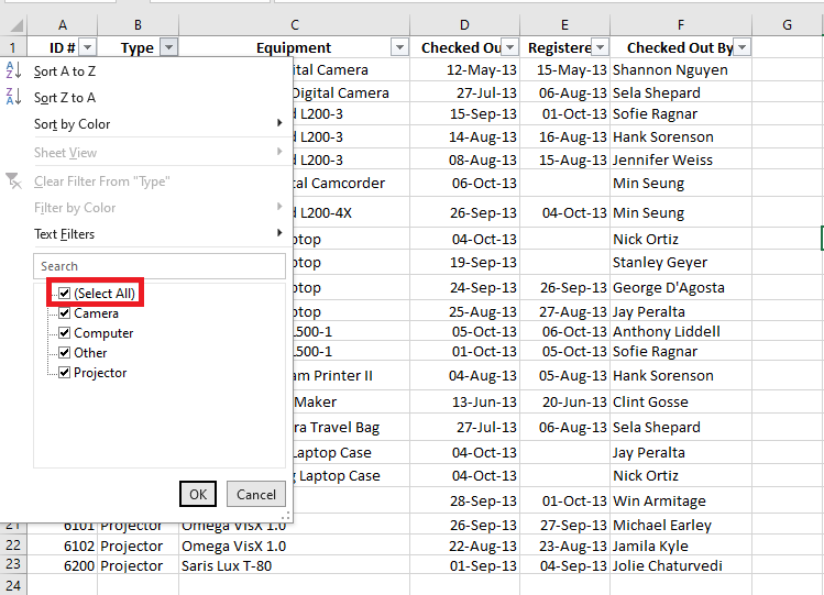
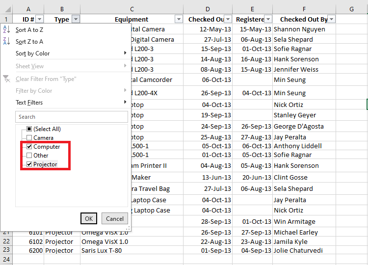
Click the dropdown arrow in the column you wish to filter. For instance, filter Column B to display only specific equipment types.
-
The filter menu will appear.
-
Uncheck “Select All” to quickly deselect everything.
-
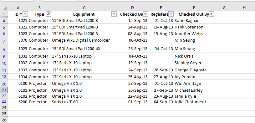
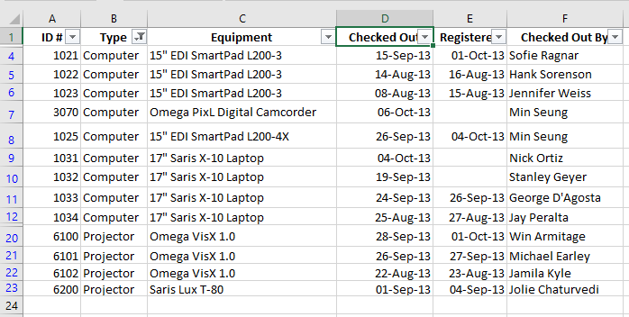
Then, check only the options you wish to display — in this example, “Laptop” and “Projector”. Click OK.
-
Excel will now hide all rows that do not match the selected values, making only laptops and projectors visible.
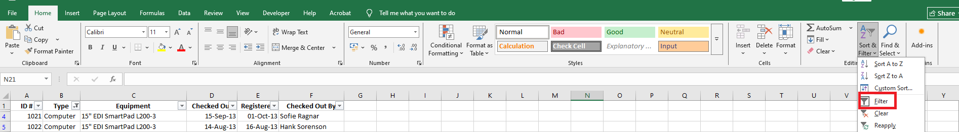
You can also access filtering options via the Home tab under the “Sort & Filter” group.
Applying Multiple Filters
Excel allows cumulative filtering, meaning you can apply multiple filters across different columns to narrow down results even further.
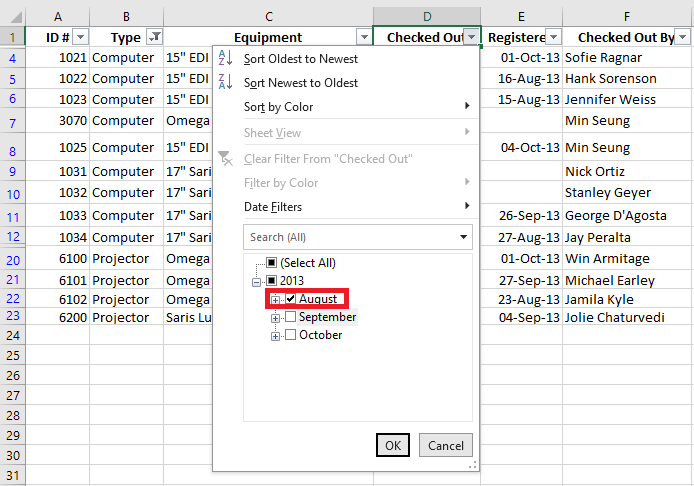
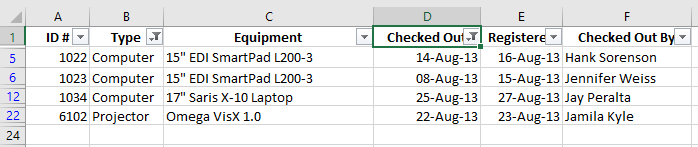
Let’s say the sheet is already filtered to show only laptops and projectors, and now you want to display only those items that were checked out in August:
-
Click the dropdown arrow in the Date column (e.g., Column D).
-
The filter menu appears.
-
Deselect all other months except August, then click OK.
-
Your spreadsheet will now show only laptops and projectors that were checked out in August.
Clearing Filters
Once you’re done analyzing, you may want to remove filters:
-
Click the dropdown arrow of the filtered column (e.g., Column D).
-
Choose Clear Filter From [Column Name].

-
All previously hidden rows will reappear.
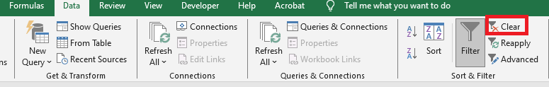
To remove all filters in one click, go to the Data tab, click on the Filter command, and then choose Clear.
Using Advanced Filtering Options
If basic filters aren’t sufficient, Excel provides advanced filtering tools like search, text filters, date filters, and number filters to help pinpoint specific data.
Filtering with the Search Box
Let’s say you want to view only equipment from the brand “Saris”:
-
Click the dropdown arrow in the Brand column (e.g., Column C).
-
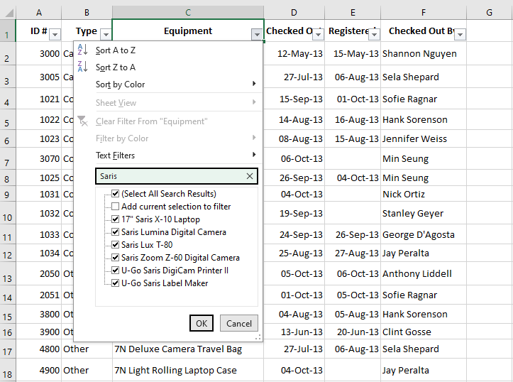
In the search box, type Saris.
-
Excel will dynamically display matching options. Select them and click OK.
-
The sheet will now show only rows containing the brand “Saris”.
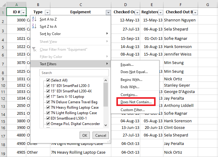
Using Advanced Text Filters
Text filters allow for even more control. For example, to exclude all items containing the word Laptop:
-
Click the dropdown arrow in Column C.
-
Hover over Text Filters and select Does Not Contain…
-
In the dialog box, type Laptop and click OK.
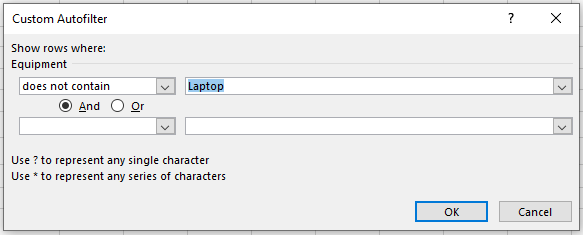
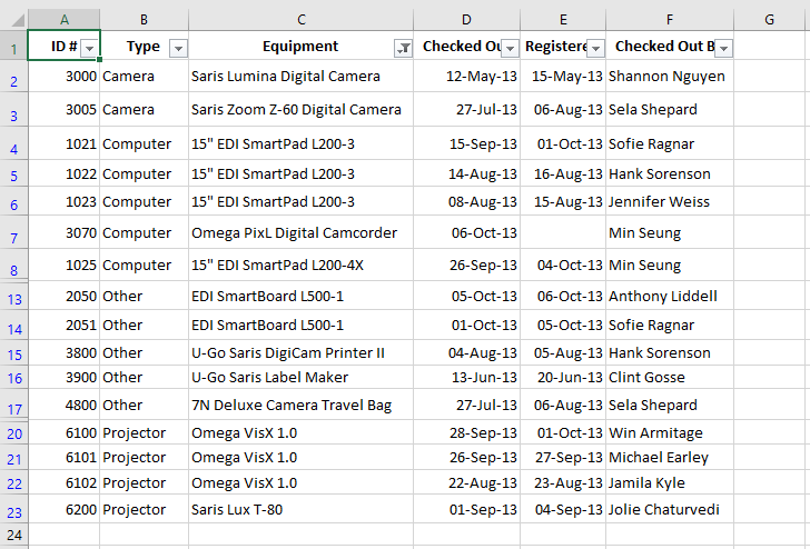
-
The filtered view will now exclude any item that contains the word “Laptop”.
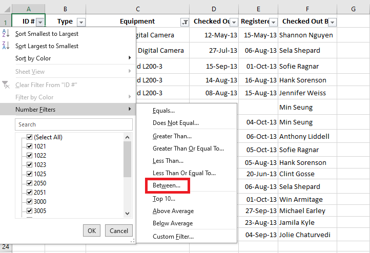
Using Advanced Number Filters
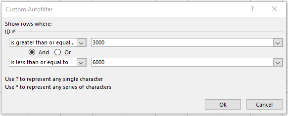
To display equipment with ID numbers between 3000 and 6000:
-
Click the dropdown in the ID# column (A).
-
Hover over Number Filters, and choose Between…
-
Enter 3000 and 6000, then click OK.
-
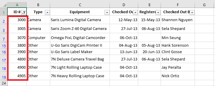
Excel will now display only items with IDs in the specified range.
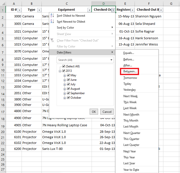
Using Advanced Date Filters
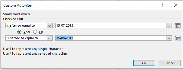
To filter equipment retrieved between July 15 and August 15:
-
Click the dropdown arrow in the Date column (D).
-
Hover over Date Filters, and choose Between…
-
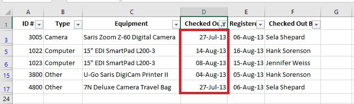
Enter 15-07-2013 and 15-08-2013 (or in your local format), then click OK.
-
The spreadsheet will display only items retrieved within this date range.
These filtering techniques are powerful tools for managing large datasets efficiently in Excel. Whether you’re dealing with text, numbers, or dates, filters allow you to quickly extract meaningful insights from your data.