Use the LEFT and RIGHT functions to split a text string of digits
A worksheet contains a list of 10-digit numbers that need to be split into two parts: a three-digit part and a seven-digit part. Use the LEFT and RIGHT functions to do this. The LEFT function returns the first character(s) in a text string, based on the number of characters specified. The RIGHT function returns the last character(s) in a text string based on the number of characters specified.
Syntax of the LEFT function:
LEFT(text, [num_chars])
The LEFT function has the following arguments:
■ text (Required). The text string that contains the characters you want to extract.
■ num_chars (Optional). Specifies the number of characters to return.
- num_chars must be greater than or equal to zero.
- If num_chars is greater than the length of text, the function returns the entire text.
- If omitted, the default value of num_chars is 1.
Syntax of the RIGHT function:
RIGHT(text, [num_chars])
The RIGHT function includes the following arguments:
■ text (Required). The text string that contains the characters you want to extract.
■ num_chars (Optional). The number of characters to return.
- Must be greater than or equal to zero.
- If it exceeds the length of text, the entire text is returned.
- If omitted, the default is 1.
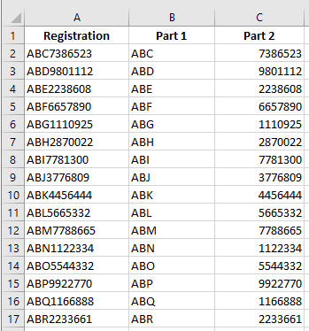
To split a string of digits:
- In a worksheet, enter a series of 10-character numbers in cells A2:A17. Letters may also be included.
- Select cells B2:B17 and type:
=LEFT(A2,3) - Press Ctrl+Enter.
- Select cells C2:C17 and type:
=RIGHT(A2,7) - Press Ctrl+Enter.
Use the LEFT function to convert invalid numbers into valid ones
In this example, invalid numbers must be corrected. These numbers contain a minus sign at the end.
Excel cannot interpret this correctly, so the minus sign must be moved to the left of the number.
First, use the LEN function to determine the length of each number. Then use LEFT to shift the minus sign.
Syntax of the LEN function:
LEN(text)
■ text (Required). The text whose length you want to determine. Spaces count as characters.
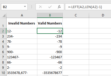
To cut the last character and display a negative value:
- Enter a series of numbers with a trailing minus sign in cells A2:A10.
- Select B2:B10 and enter:
= -LEFT(A2, LEN(A2)-1) - Press Ctrl+Enter.
Use the FIND function to split the first name from the last name
This task shows how to separate first and last names. Full names are listed in column A.
We want to extract the first name into column B. The FIND function can locate the space separating the two parts.
Syntax:
FIND(find_text, within_text, [start_num])
■ find_text: The character or text to locate. You can use wildcards: ? (any single character), * (any sequence). Use ~ before a wildcard to search for the literal character.
■ within_text: The text where you search.
■ start_num: The position to start the search. Default is 1.
Examples:
=FIND("n", "printer") returns 8
=FIND("form", "platform") returns 6
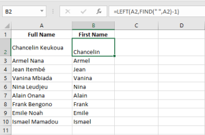
To extract the first name:
- Enter full names in A2:A10.
- Select B2:B11 and type:
=LEFT(A2, FIND(" ", A2)-1) - Press Ctrl+Enter
Use the MID function to extract the last name
Full names are listed in column A. We want to extract the last name into column B.
Use FIND to identify the space, then use MID to return characters starting just after it.
Syntax:
MID(text, start_num, num_chars)
■ text (Required). The string containing the characters to extract.
■ start_num (Required). Position of the first character to extract.
- If start_num > length of text, MID returns an empty string.
- If start_num + num_chars > length, MID returns the rest of the string.
- If start_num < 1, MID returns #VALUE!
■ num_chars (Required). Number of characters to extract. - If negative, returns #VALUE!
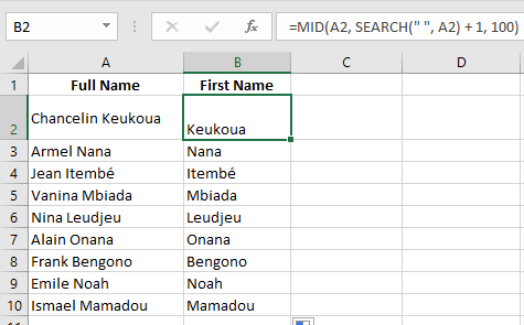
To extract the last name:
- Enter full names in A2:A10.
- Select B2:B11 and type:
=MID(A2, FIND(" ", A2)+1, 100) - Press Ctrl+Enter
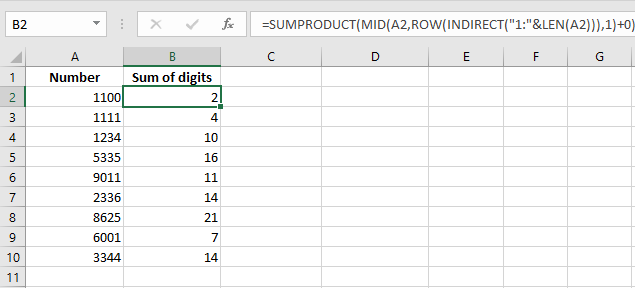
Use the MID function to sum digits in a number
The worksheet contains 4-digit numbers in column A.
We want to sum the digits of each number. Use MID to extract each digit and add them.
To calculate the digit sum:
- Enter 4-digit numbers in A2:A10.
- Select B2:B10 and enter:
=MID(A2,1,1)+MID(A2,2,1)+MID(A2,3,1)+MID(A2,4,1) - Press Ctrl+Enter
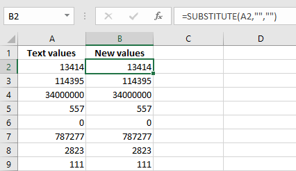
Use the SUBSTITUTE function to replace characters
Column A contains values formatted as text.
Use the SUBSTITUTE function to replace specific characters.
Syntax:
SUBSTITUTE(text, old_text, new_text, [instance_num])
■ text (Required). The string or cell reference.
■ old_text (Required). The text to be replaced.
■ new_text (Required). The replacement text.
■ instance_num (Optional). Specifies which occurrence to replace.
If omitted, all instances of old_text are replaced.
To make Excel recognize text as numbers:
- Format column A as text.
- Enter numbers (as text) in A2:A10.
- In B2:B10, enter:
=SUBSTITUTE("'" , " ")(This example seems incorrect — see note) - Press Ctrl+Enter.
- In A12:
=SUM(A2:A10) - In B12:
=SUM(B2:B10)
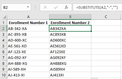
Use SUBSTITUTE to replace parts of a cell
To replace a character:
- Select B2:B9 and type:
=SUBSTITUTE(A2, "-", "", 1) - Press Ctrl+Enter
Note: To replace the second occurrence, use:
=SUBSTITUTE(A2, "-", "", 2)
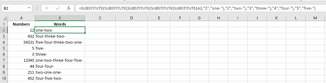
Use SUBSTITUTE to convert digits into words
The worksheet contains numbers 1 to 5 in column A.
Use nested SUBSTITUTE functions to convert them into words.
To convert digits to words:
- Enter numbers 1–5 in column A.
- In B2:B10, enter:
=SUBSTITUTE(SUBSTITUTE(SUBSTITUTE(SUBSTITUTE(SUBSTITUTE(A2,1,"one-"),2,"two-"),3,"three-"),4,"four-"),5,"five-")
Use SUBSTITUTE to remove carriage return characters
To wrap text in a cell: use the Wrap Text option or press Alt+Enter to insert line breaks.
To remove line breaks, use SUBSTITUTE with the CHAR function.
The ASCII code for line break is 10.
To remove line breaks:
- Enter multi-line text in cell A2.
- In B2, type:
=SUBSTITUTE(A2, CHAR(10), " ") - Press Ctrl+Enter
