Worksheets containing a lot of complex and detailed information can be difficult to read and analyze. Fortunately, Microsoft Excel provides a simple way to organize data into groups, allowing you to collapse and expand rows with similar content to create more compact and understandable views.
How to Group Rows
Grouping in Excel works best with well-structured worksheets that have column headers, no empty rows or columns, and a summary (subtotal) row for each subset of rows. Once your data is properly organized, use one of the following methods to group it.
Automatically Grouping Rows
If your dataset contains only one level of information, the quickest way is to let Excel group the rows for you. Here’s how:
- Select any cell in one of the rows you want to group.
- Go to the Data tab, in the Outline group, click the arrow under Group, and select Auto Outline.
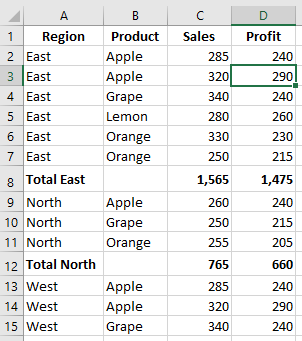
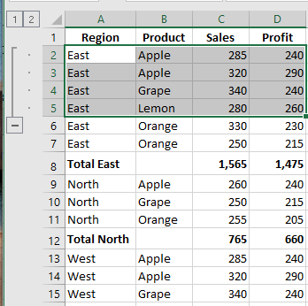
Here is an example of the type of rows Excel can group:

As shown in the screenshot below, the rows are neatly grouped, and outline bars representing different organization levels are added to the left of column A.
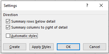
Note: If your summary rows are located above the group of detail rows, go to the Data tab > Outline group, click the Outline Settings dialog launcher, and uncheck Summary rows below detail.
Once the outline is created, you can quickly collapse or expand the details of any group by clicking the minus or plus sign of that group. You can also collapse or expand all rows at a certain level by clicking the level buttons in the upper-left corner of the worksheet.
Manually Grouping Rows
If your worksheet contains at least two levels of information, Excel’s Auto Outline may not group your data correctly. In that case, you can manually group rows by doing the following.
Note: When manually outlining, make sure your dataset does not contain any hidden rows, or your data may be grouped incorrectly.
Create Outer Groups (Level 1)
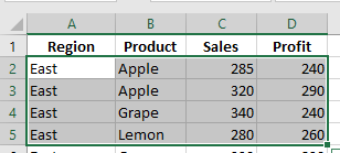
Select one of the largest subsets of data, including all intermediate summary rows and their detail rows. In the example below, to group all data under row 9 (« East Total »), we select rows 2 to 8.
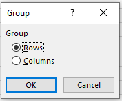
On the Data tab, in the Outline group, click the Group button, select Rows, then click OK.
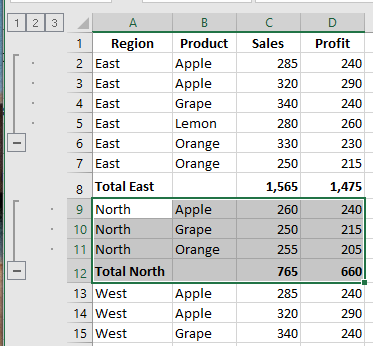
Do the same to create as many outer groups as needed. In this example, we create another outer group for the North region by selecting rows 9 to 12 and clicking Data > Group > Rows:
Tip: To create a new group faster, press Shift + Alt + Right Arrow instead of clicking the Group button on the ribbon.
Create Nested Groups (Level 2)
To create an inner group, select all the detail rows above the related summary row, then click the Group button. For example, to group “Apples” in the East region, select rows 2 and 3 and press Group. Then group “Oranges” by selecting rows 5 to 7. Do the same for the North region:
Add More Grouping Levels If Needed
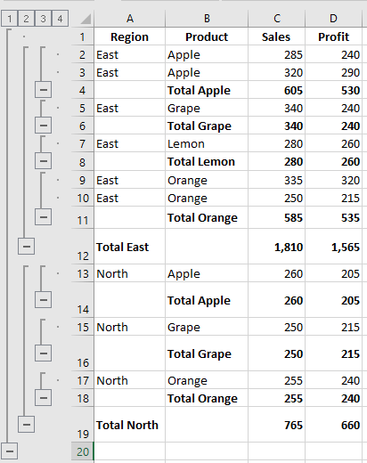
Datasets are rarely final. If you add more data, you may want to insert more outline levels. For instance, after inserting a Grand Total row, select all rows except the Grand Total row (rows 2 to 17), and then click Data > Group > Rows. Now your data has 4 levels:
- Level 1: Grand Total
- Level 2: Region totals
- Level 3: Item subtotals
- Level 4: Detail rows
Now that we’ve outlined the rows, let’s see how this helps with data visualization.
How to Collapse Rows
One of the most useful features of Excel grouping is the ability to hide or show detail rows for a specific group, or collapse/expand the entire outline to a particular level with a single mouse click.
Collapse Rows Within a Group
To collapse the rows of a particular group, simply click the minus sign at the bottom of the group’s outline bar. For example, to hide all detail rows for the East region and show only the « East Total » row:
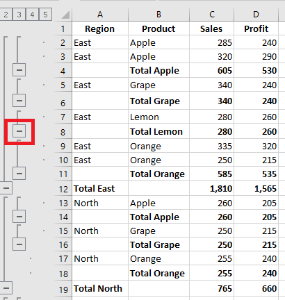
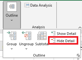
Another way is to select any cell in the group and click Hide Detail on the Data tab in the Outline group:
In either case, the group will collapse to just the summary row, and all detail rows will be hidden.
Collapse or Expand the Entire Outline at a Specific Level
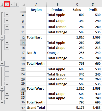
To collapse or expand all groups to a specific level, click the corresponding level number in the upper-left corner of your worksheet. Level 1 shows the least data, while higher numbers expand more rows.
In our dataset with 4 outline levels:
- Level 1: Shows only the Grand Total (row 18)
- Level 2: Grand Total + Regional Totals (rows 9, 17, 18)
- Level 3: Adds Item Subtotals (rows 4, 8, 13, 16)
- Level 4: Shows all detail rows
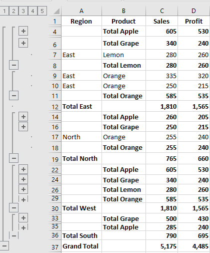
The screenshot below shows the outline collapsed to level 3:
How to Expand Rows in Excel
To expand a specific group, click any cell in the summary row and then click Show Detail on the Data tab in the Outline group:
Or click the plus sign for the collapsed group you want to expand:
How to Remove the Outline
If you want to remove all grouped rows at once, clear the outline. If you want to remove only specific groups (like nested ones), ungroup the selected rows.
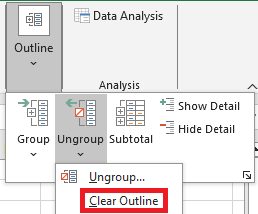
To remove the entire outline:
- Go to the Data tab > Outline group
- Click the arrow under Ungroup, then click Clear Outline
Notes:
- Removing an outline does not delete any data.
- If you clear an outline with collapsed rows, those rows may remain hidden.
- Once the outline is removed, you cannot undo it with Undo (Ctrl + Z). You must recreate the outline from scratch.
How to Ungroup Specific Rows
To remove grouping from certain rows without deleting the entire outline:
- Select the rows you want to ungroup.
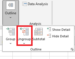
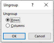
- Go to Data > Outline, click Ungroup or press Shift + Alt + Left Arrow (Excel’s Ungroup shortcut).
- In the Ungroup dialog box, select Rows and click OK.
For example, here’s how to ungroup two nested groups (Apples Subtotal and Oranges Subtotal) while keeping the outer « East Total » group:
Note: You cannot ungroup non-adjacent row groups at once. Repeat the steps for each group individually.
How to Automatically Calculate Group Subtotals
In the above examples, we inserted our own subtotal rows with SUM formulas. To have Excel calculate subtotals automatically, use the Subtotal command with a summary function such as SUM, COUNT, AVERAGE, MIN, MAX, etc.
The Subtotal command will insert summary rows and create an outline with collapsible/expandable rows — two tasks in one!
Applying Excel’s Default Styles to Summary Rows
Microsoft Excel provides predefined styles for two levels of summary rows: RowLevel_1 (bold) and RowLevel_2 (italic). You can apply these styles either before or after grouping the rows.
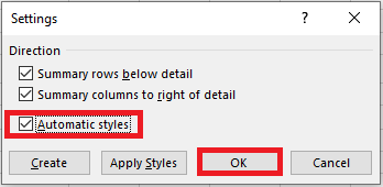
To automatically apply styles to a new outline:
- Go to Data > Outline
- Click the Outline Settings dialog launcher
- Check the Automatic Styles box and click OK
To apply styles to an existing outline, check the same box and click Apply Styles instead of OK.
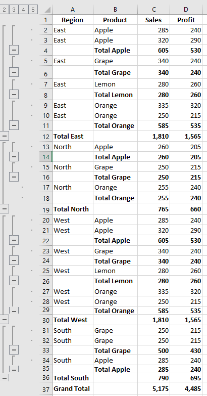
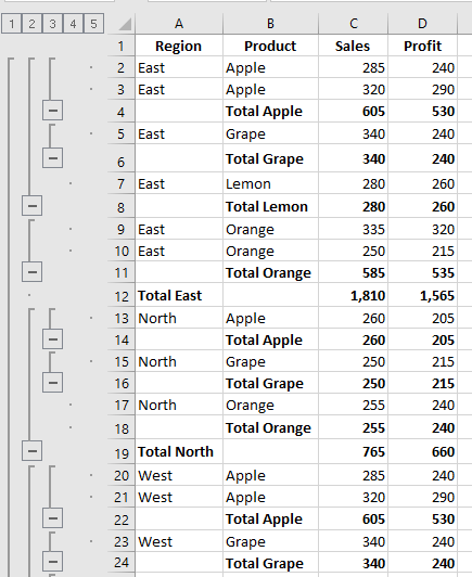
Here’s what an outlined sheet looks like with default summary row styles:
How to Select and Copy Only Visible Rows
After collapsing unnecessary rows, you may want to copy only the visible (relevant) data. However, selecting rows the usual way with the mouse also selects hidden rows.
To select only visible rows:
- Select the visible rows using the mouse (e.g., only summary rows).
- Go to Home > Editing > Find & Select > Go To Special
Or press Ctrl + G, then click Special… - In the Go To Special dialog box, select Visible cells only and click OK.
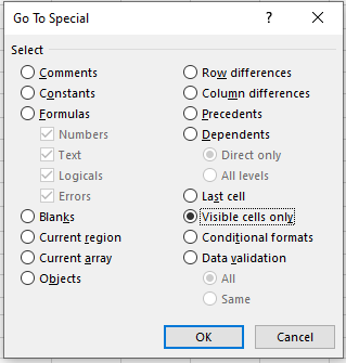
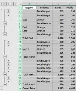
Only visible rows are now selected (adjacent to hidden ones marked with white borders):
Now press Ctrl + C to copy and Ctrl + V to paste wherever you want.
How to Show or Hide Outline Symbols
To toggle the display of outline symbols and level numbers, use the shortcut Ctrl + 8. Press once to hide the symbols, press again to show them.
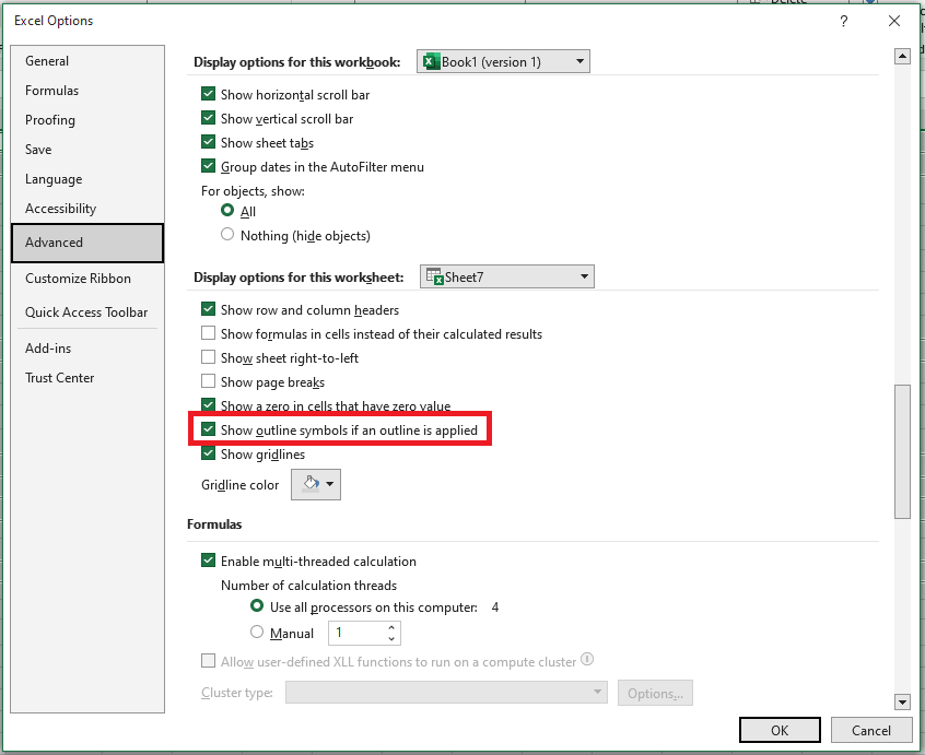
If you do not see the plus/minus symbols or level numbers, check this setting:
- Go to File > Options > Advanced
- Scroll to Display options for this worksheet
- Select your worksheet and ensure Show outline symbols if an outline is applied is checked.
This is how you group rows in Excel to collapse or expand sections of your dataset. Likewise, you can group columns in your worksheets.