
In mathematics, the average (more precisely the arithmetic mean) is calculated by summing a group of numbers and then dividing that total by the count of the numbers.
For example, if three athletes complete a race in 10.5 seconds, 10.7 seconds, and 11.2 seconds respectively, the average time would be:
= (10.5 + 10.7 + 11.2) / 3,
which gives 10.8 seconds.
However, in Excel, you don’t need to write this kind of mathematical expression manually. Excel provides powerful built-in functions such as AVERAGE() that automatically handle these calculations.
AVERAGE() Function
The AVERAGE() function in Excel returns the arithmetic mean of the specified numbers. Its syntax is:
=AVERAGE(number1, [number2], …)
- number1, number2, etc., are the values you want to average. The first argument is required, and up to 255 arguments are allowed.
- These values can be numbers, cell references, or ranges.
How to Use AVERAGE()
The AVERAGE() function is one of the simplest and most frequently used in Excel. Here are some practical examples:
- To calculate the average of numbers directly:
=AVERAGE(1, 2, 3, 4) → returns 2.5 - To average an entire column:
=AVERAGE(A:A) - To average an entire row:
=AVERAGE(1:1) - To average a specific range:
=AVERAGE(B2:B11)
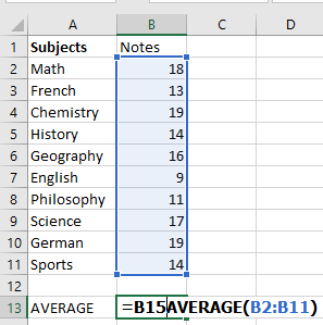
Without the AVERAGE function, you’d have to manually input:
=(B2+B3+B4+…+B11)/10,
or use:
=SUM(B2:B11)/COUNT(B2:B11)
You can also average non-contiguous cells:
=AVERAGE(A1, C1, D1)
Mixed input types (ranges, values, references) are supported:
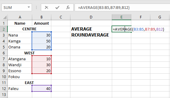
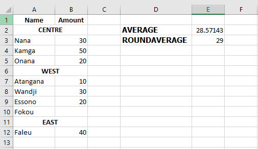
=AVERAGE(B3:B5, B7:B9, B12)
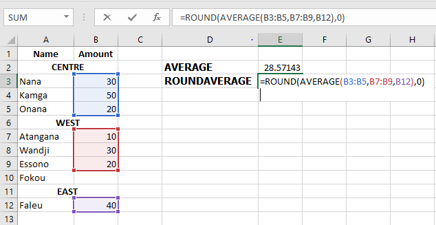
To round the result to the nearest whole number:
=ROUND(AVERAGE(B3:B5, B7:B9, B12), 0)
You can also average percentages or times.
Important: The AVERAGE() function includes zero values. If you want to ignore zeros, use AVERAGEIF() instead.
AVERAGE() – Key Notes
- Zeros are included in the average.
- Empty cells, text, Boolean values (TRUE, FALSE) are ignored—unless typed directly in the formula, in which case TRUE=1, FALSE=0.
- Distinguish between zero and an empty cell: zeros are counted, blanks are not. This is affected by the « Show a zero in cells that have zero value » Excel setting (File > Options > Advanced).
AVERAGEA() Function
AVERAGEA() works like AVERAGE() but includes all non-empty cells, including:
- Numbers
- Text (treated as 0)
- Logical values (TRUE = 1, FALSE = 0)
=AVERAGEA(value1, [value2], …)
Examples:
- =AVERAGEA(2, FALSE) → returns 1
- =AVERAGEA(2, TRUE) → returns 1.5
AVERAGEIF() Function
AVERAGEIF() calculates the average of cells that meet a specific condition.
Syntax:
=AVERAGEIF(range, criteria, [average_range])
Where:
- range: cells to test
- criteria: the condition
- average_range (optional): cells to average if different from range
Examples:
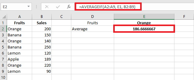
Exact match:
=AVERAGEIF(A2:A9, « Orange », B2:B9)
Or using a cell reference:
=AVERAGEIF(A2:A9, E1, B2:B9)
Rounded result:
=ROUND(AVERAGEIF(A2:A9, « Orange », B2:B9), 2)
Partial match (wildcards):
- * for any sequence
- ? for a single character
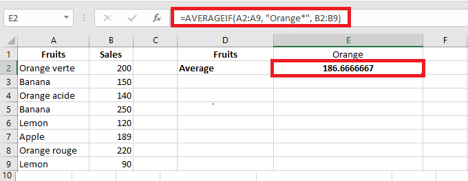
E.g., average all « Orange »-related items:
=AVERAGEIF(A2:A9, « Orange* », B2:B9)
Exclude « Orange »:
=AVERAGEIF(A2:A9, « <>*Orange* », B2:B9)
Numeric conditions:
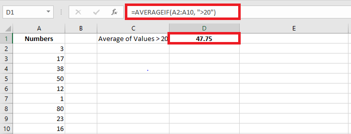
Average values greater than 20:
=AVERAGEIF(A2:A10, « >20 »)
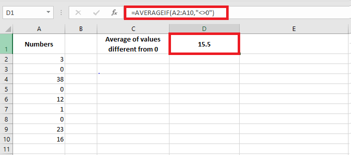
Exclude zeros:
=AVERAGEIF(A2:A10, « <>0 »)
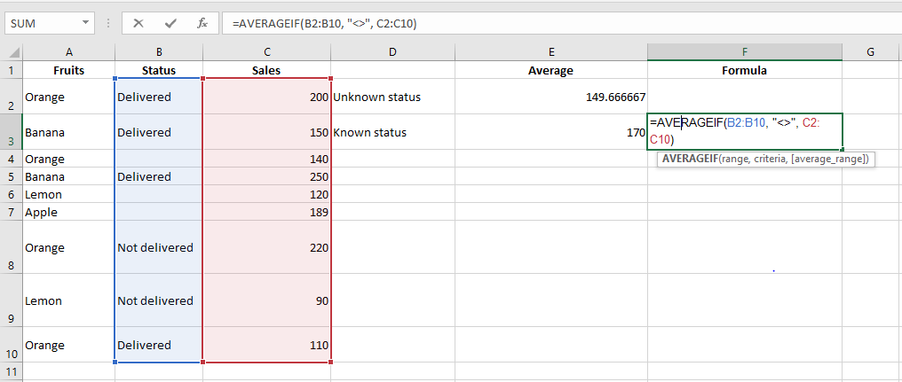
Empty/non-empty cells:
- Empty: =AVERAGEIF(B2:B10, « = », C2:C10)
- Textually blank (e.g. = » »): =AVERAGEIF(B2:B10, « », C2:C10)
- Non-empty: =AVERAGEIF(B2:B10, « <> », C2:C10)
AVERAGEIFS() Function
AVERAGEIFS() averages cells that meet multiple conditions (AND logic).
Syntax:
=AVERAGEIFS(average_range, criteria_range1, criteria1, [criteria_range2, criteria2], …)
Examples:
Multiple conditions:
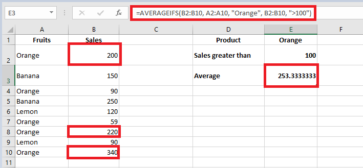
Average sales of « Orange » where sales > 100:
=AVERAGEIFS(B2:B10, A2:A10, « Orange », B2:B10, « >100 »)
Date conditions:
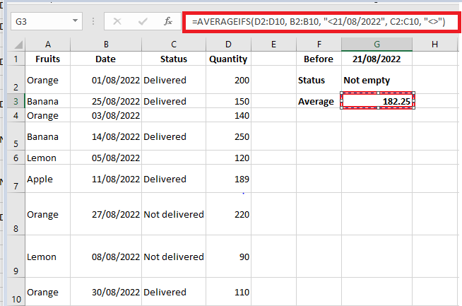
Average quantity delivered before 21-Aug-2022 with a non-empty status:
=AVERAGEIFS(D2:D10, B2:B10, « <21/08/2022 », C2:C10, « <> »)
Important Notes on AVERAGEIF and AVERAGEIFS
- Empty or non-numeric cells in average_range are ignored.
- If no cells match criteria, the result is #DIV/0!.
- In AVERAGEIF(), the average_range doesn’t need to match the size of the range, but the top-left cell determines alignment.
- In AVERAGEIFS(), all criteria ranges must match the size of average_range.
How to Average with OR Logic (Multiple Conditions)
Since AVERAGEIFS() uses AND logic, to apply OR logic, you’ll need custom formulas.
Example 1: OR logic with text values
Average sales of « Banana » or « Apple »:
=AVERAGE(IF(ISNUMBER(MATCH(A2:A8, {« Banana », « Apple »}, 0)), B2:B8))
Or using cell references (e.g. E1:E2 contain « Banana » and « Apple »):
=AVERAGE(IF(ISNUMBER(MATCH(A2:A8, E1:E2, 0)), B2:B8))
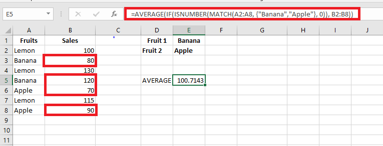
Press Ctrl + Shift + Enter to confirm (array formula).
Example 2: OR logic with numeric conditions
Average sales in column D where either column C or D > 50:
=SUM(IF(((C2:C8>50)+(D2:D8>50))>0, D2:D8, 0)) / SUM(–((C2:C8>50)+(D2:D8>50)>0))
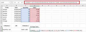
Adaptable for different thresholds, e.g. D2:D8>100.
Example 3: OR logic with empty/non-empty cells
Non-empty cells in column B or C:
=SUM(IF(((B2:B8<> » »)+(C2:C8<> » »))>0, D2:D8, 0)) / SUM(–(((B2:B8<> » »)+(C2:C8<> » »))>0))
Empty cells in column B or C:
=SUM(IF(((B2:B8= » »)+(C2:C8= » »))>0, D2:D8, 0)) / SUM(–(((B2:B8= » »)+(C2:C8= » »))>0))
Conclusion
Excel offers powerful and flexible ways to calculate averages using functions like AVERAGE(), AVERAGEA(), AVERAGEIF(), and AVERAGEIFS(). You can also craft custom formulas to implement OR logic or handle special cases such as blank cells and conditional criteria. With the right understanding, you can efficiently analyze your data in virtually any scenario.