This function returns values of the cumulative beta distribution, which is commonly used to analyze variance across samples (e.g., modeling proportions like daily computer usage time).
Syntax:
BETA.DIST(x; alpha; beta; cumulative; [A]; [B])
Arguments:
- x (required): The value (between A and B) to evaluate.
- alpha (required): A shape parameter of the distribution.
- beta (required): A second shape parameter.
- cumulative (required): A logical value (TRUE = cumulative probability; FALSE = probability density).
- A (optional): Lower bound for x (default = 0).
- B (optional): Upper bound for x (default = 1).
Background
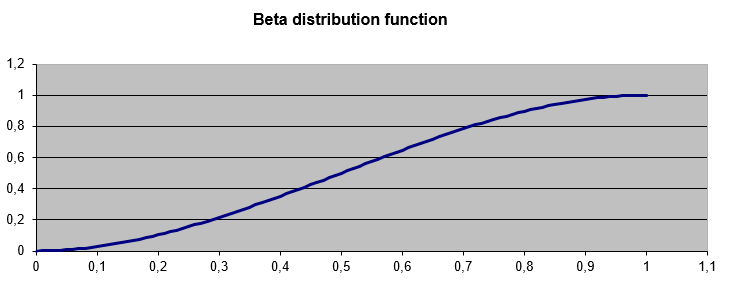
- The beta distribution models probabilities for variables bounded within a fixed interval (e.g., 0 to 1).
- alpha and beta control the distribution’s shape (see Figure below).
- If A and B are omitted, x must be between 0 and 1.
Example
Question:
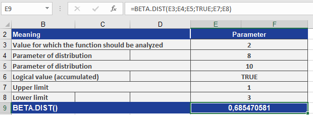
What is the cumulative probability of x = 2 for a beta distribution with:
- Shape parameters alpha = 8, beta = 10
- Bounds A = 1, B = 3?
Formula:
BETA.DIST(2, 8, 10, TRUE, 1, 3)
Result: 0.68547 (see Figure below).
Interpretation:
There is a 68.547% probability that a randomly selected value from this distribution falls between 1 and 2.
Key Notes
- Bounds: If A and B are specified, x must lie within [A, B].
- Cumulative vs. Density:
- TRUE: Returns the cumulative distribution (area under the curve up to x).
- FALSE: Returns the probability density at x.
- Applications: Useful for modeling proportions (e.g., task completion rates, survey responses).