This function returns the inverse of the beta cumulative distribution. Given a probability, it finds the corresponding value x such that:
- If probability = BETA.DIST(x, …), then BETA.INV(probability, …) = x.
Syntax
BETA.INV(probability; alpha; beta; [A]; [B])
Common Use Case:
- In project planning, it estimates completion times based on expected duration and variance.
Arguments
| Argument | Required? | Description |
| probability | Yes | A probability (0 ≤ probability ≤ 1) linked to the beta distribution. |
| alpha | Yes | Shape parameter (must be > 0). |
| beta | Yes | Shape parameter (must be > 0). |
| A | No | Lower bound (default = 0). |
| B | No | Upper bound (default = 1). |
Note: If A is specified, B must also be provided.
Background
- Beta Distribution Basics:
- Models continuous probabilities for variables bounded in [0, 1].
- Defined by shape parameters alpha (p) and beta (q).
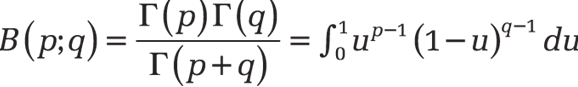
- Probability Density Function :
-
-
- B(p, q) = Beta function (normalization factor).
- Γ(p) = Gamma function.
-
- Key Properties:
- Expected Value: E[X] = alpha / (alpha + beta)
- Variance: Var(X) = (alpha * beta) / [(alpha + beta)^2 * (alpha + beta + 1)]
- Inverse Function:
- BETA.INV() reverses BETA.DIST(), returning the quantile x for a given probability.
Example
Problem:
- Given a beta distribution with:
- Shape parameters: alpha = 8, beta = 10
- Bounds: A = 1, B = 3
- What value x corresponds to a cumulative probability of 0.68547?
Formula:
BETA.INV(0.685470581, 8, 10, 1, 3)
Result: 2 (see Figure below).
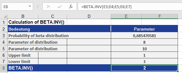
Interpretation:
- There is a 68.547% probability that a random variable from this distribution falls below 2 (within the range [1, 3]).
Key Notes
- Bounds Adjustment:
- If A and B are provided, the result scales linearly from [0, 1] to [A, B].
- Applications:
- Project Management: Estimating task durations (PERT analysis).
- Statistics: Modeling proportions (e.g., conversion rates, survey responses).
- Error Handling:
- Returns #NUM! if probability ≤ 0 or ≥ 1, or if alpha/beta ≤ 0.