This function returns the inverse of the right-tailed chi-square (χ²) distribution, providing the critical value where:
- If probability = CHISQ.DIST.RT(x, df), then CHISQ.INV.RT(probability, df) = x.
Syntax
CHISQ.INV.RT(probability; degrees_freedom)
Purpose
Used in hypothesis testing to:
- Determine critical values for χ² tests (e.g., goodness-of-fit, independence).
- Validate whether observed results significantly deviate from expected results under the null hypothesis.
Arguments
| Argument | Required? | Description |
| probability | Yes | Right-tailed probability (α) associated with the χ²-distribution (e.g., 0.05 for 5% significance). |
| degrees_freedom | Yes | Degrees of freedom (positive integer). For contingency tables: (rows – 1) * (columns – 1). |
Background
- Right-Tailed χ² Distribution:
- Models the sum of squared deviations from expected values.
- Used when testing « greater than » hypotheses (e.g., variance exceeds a threshold).
- Key Concepts:
- Critical Value (x):
- The χ² value beyond which the null hypothesis is rejected.
- Calculated as CHISQ.INV.RT(α, df).
- Degrees of Freedom (df):
- Depends on the test type. For a 2×2 contingency table, df = 1.
- Critical Value (x):
- Inverse Relationship:
- CHISQ.INV.RT(α, df) is the inverse of CHISQ.DIST.RT(x, df).
Example: Vitamin C Efficacy Study
Scenario
- Goal: Test if Vitamin C reduces cold risk (null hypothesis: no effect).
- Data:
- Expected cold cases (no Vitamin C): 22/936.
- Observed cold cases (Vitamin C group): Fewer than 22.
- Significance Level (α): 2.5% (one-tailed test).
Step 1: Calculate Critical Value
CHISQ.INV.RT(0.025; 1) // Returns 5.0239
- Interpretation: If the test statistic (v) > 5.0239, reject the null hypothesis.

Step 2: Compute Test Statistic (v)
- For each category, calculate:
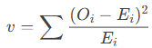
-
- Oi = Observed frequency.
- Ei = Expected frequency.
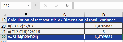
- Result: Suppose v = 6.47 (see Figure below).
Step 3: Compare v to Critical Value
- 6.47 > 5.0239 → Reject the null hypothesis.
- Conclusion: Insufficient evidence to confirm Vitamin C reduces colds at α = 2.5%.
Key Notes
- When to Use:
- Goodness-of-Fit Tests: Compare observed vs. expected frequencies.
- Independence Tests: Check if two categorical variables are related.
- Degrees of Freedom:
- For a contingency table: df = (rows – 1) * (columns – 1).
- For variance tests: df = sample size – 1.
- Common Errors:
- #NUM! if:
- probability ≤ 0 or ≥ 1.
- degrees_freedom < 1.
- #NUM! if: