This function performs a chi-square (χ²) test of independence, returning the p-value associated with the test statistic. It compares observed frequencies (actual_range) against expected frequencies (expected_range) to determine if there is a statistically significant association between categorical variables.
Syntax
CHISQ.TEST(actual_range; expected_range)
Arguments
| Argument | Required? | Description |
| actual_range | Yes | Range of observed frequencies (e.g., survey counts). |
| expected_range | Yes | Range of expected frequencies under the null hypothesis. |
Note:
- Ranges must have the same dimensions. If not, #N/A is returned.
- Expected frequencies should ideally be ≥5 for reliable results.
Background
- Chi-Square Test Statistic (χ²):
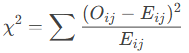
-
- Oij = Observed frequency in row ii, column jj.
- Eij= Expected frequency (calculated from row/column totals).
- Degrees of Freedom (df):
- For an r×cr×c contingency table:
df=(r−1)(c−1)df=(r−1)(c−1)
- Null Hypothesis (H₀):
- Assumes no association between variables (observed ≈ expected).
- Low p-value (e.g., <0.05): Reject H₀ (significant association).
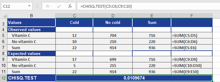
Example: Vitamin C and Colds Study
Scenario
- Goal: Test if Vitamin C usage affects cold incidence.
- Data:
- Observed (actual_range): 22 colds in 936 Vitamin C users.
- Expected (expected_range): 30 colds (baseline rate without Vitamin C).
Step 1: Run CHISQ.TEST()
CHISQ.TEST(A2:A3; B2:B3) // Returns p-value = 0.01 (1%)
*(See Figure below for setup.)*
Step 2: Interpret Results
- p-value = 0.01:
- 1% probability that the deviation (observed vs. expected) is due to chance.
- Conclusion: Reject H₀ at 99% confidence (Vitamin C likely reduces colds).
Key Outputs
| Metric | Value | Interpretation |
| χ² Statistic | Calculated | Higher = greater deviation. |
| Degrees of Freedom | 1 | (2×2 table: (2-1)(2-1)=1). |
| p-value | 0.01 | Significant at α=0.05. |
Key Notes
- When to Use:
- Goodness-of-fit: Compare observed vs. theoretical distributions.
- Independence tests: Check if two categorical variables are related (e.g., gender vs. product preference).
- Limitations:
- Small expected frequencies: May violate test assumptions (use Fisher’s Exact Test if any Eij<5Eij<5).
- Binary outcomes: For 2×2 tables, consider Yates’ correction for continuity.
- Follow-up Analysis:
- If significant, calculate Cramer’s V or Phi coefficient to measure association strength.