This function uses an index to return a value from the list of value arguments.
Syntax:
CHOOSE(index; value1; value2; …)
Arguments:
- index (required): Specifies which item is selected from the value arguments.
- value1, value2, … (the first value argument is required): A list of values separated by commas. These can be numbers, cell references, defined names, formulas, functions, or text.
- In Excel the maximum number of arguments is 254.
- In earlier versions, the limit is 29.
Background:
- The index argument must evaluate to an integer between 1 and 29 (or 1 and 254, depending on the Excel version).
- You can use a formula or a cell reference that returns such a number.
- If index is less than 1 or greater than the number of value arguments, CHOOSE() returns the #VALUE! error.
- If index is a fraction, the decimal part is truncated before evaluation.
Using CHOOSE() in Array Formulas:
You can use CHOOSE() in an array formula by specifying the index as an array. However, be cautious to avoid errors.
- The formula:
{=CHOOSE({1;2}; SUM(E41:G41); SUM(E42:G42))}
Returns:
-
- The sum of E41:G41 in the first cell.
- The sum of E42:G42 in the second cell.
- The formula:
{=SUM(CHOOSE({1;2}; E41:G41; E42:G42))}
Returns the total of E41:G42 in both cells.
- The formulas:
=SUM(CHOOSE(1; E41:G41; E42:G42))
and
=SUM(CHOOSE(2; E41:G41; E42:G42))
Return the correct individual sums.
Example:
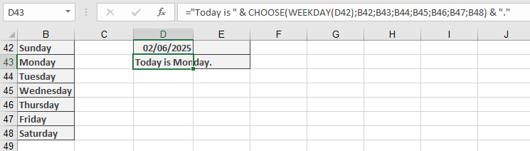
Assume the names of the days (starting with Sunday) are in cells B42:B48. The formula:
= »Today is » & CHOOSE(WEEKDAY(D42); B42; B43; B44; B45; B46; B47; B48) & « . »
Returns:
« Today is [weekday name]. »