How to use the F.INV.RT() function in Excel

The F.INV.RT() function returns the inverse of the right-tailed F-distribution. If p = F.DIST.RT(x,…), then F.INV.RT(p,…) = x.

The F-distribution is used in an F-test to compare variances between two data sets. For example, you could analyze income distributions in the United States and Canada to determine whether the two countries exhibit similar income diversity.

Syntax

F.INV.RT(probability; degrees_freedom1; degrees_freedom2)

Arguments

• probability (required): The probability associated with the F-distribution (e.g., significance level α).
• degrees_freedom1 (required): The degrees of freedom in the numerator.
• degrees_freedom2 (required): The degrees of freedom in the denominator.

Background

• The output of an ANOVA (Analysis of Variance) often includes:
  • The F-statistic
  • The F-probability (p-value)
  • The critical F-value at a specified significance level (e.g., 0.05).
• This function helps test whether the means of two or more samples are statistically equal.
• It evaluates if observed differences in group means are significant or due to random variation.

The F.INV.RT() function calculates the critical F-value for a given significance level (α). By comparing this critical value to the calculated F-statistic, you can accept or reject the null hypothesis.

Example

Scenario:
You are an occupational therapist studying how strongly employees identify with their company.

• Sample: 15 employees, each answering 10 questions (with 3 answer options per question).
• Data is summarized (Figure below).

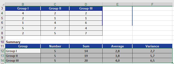
Hypotheses:

• Null hypothesis (H₀): No difference exists between the three employee groups.
• Alternative hypothesis (H₁): A significant difference exists.
• Significance level (α): 0.05 (5%).

ANOVA Results (Figure below):

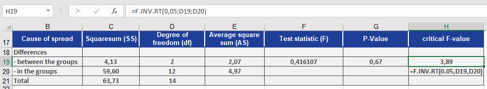
• Between-group variance: Measures differences across groups.
• Within-group variance: Measures random differences among individuals in the same group.

Degrees of Freedom:

• df1 (within groups): (5–1) + (5–1) + (5–1) = 12
• df2 (between groups): 3 groups – 1 = 2

Key Calculations:

1. F-statistic: 0.42 (cell F19).
2. Critical F-value: Calculated via F.INV.RT(0.05, 2, 12).

Conclusion:

• If the F-statistic ≥ Critical F-value, reject H₀.
• Here, 0.42 < Critical Value → H₀ is accepted.
• Interpretation: No significant difference exists between the groups.

Key Notes

• F.INV.RT() computes the threshold F-value for a given α.
• Compare this critical value to your F-statistic to decide on H₀.
• Retain H₀ if F-statistic < Critical Value (no significant difference).