
This function retrieves data from a PivotTable report. You can use GETPIVOTDATA() to extract summarized data from a PivotTable report, provided that the summary data is visible within the report.
Syntax
GETPIVOTDATA(data_field; pivot_table; field1; item1; field2; item2; …)
Arguments
- data_field (required): The name, enclosed in quotation marks, of the data field that contains the data you wish to retrieve.
- pivot_table (required): A reference to a cell, cell range, or named cell range within a PivotTable report. This information helps to identify which PivotTable report contains the data you want.
- field1, item1, field2, item2, …: You must provide at least 1 and up to 14 pairs of field names and item names that describe the specific data you want to retrieve. These pairs can be in any order. Field names and item names (except for dates and numbers) must be enclosed in quotation marks. For OLAP (Online Analytical Processing) PivotTable reports, the items can include both the source name of the dimension and the source name of the item. An example of a field and item pair for an OLAP PivotTable might look like this: « [Product] », »[Product].[All Products].[Foods].[Baked Goods] ».
Background
The PivotTable in Excel is a powerful tool for data analysis. It allows you to sort data from a database and display summarized information. You can group, hide, filter, or evaluate your data without altering the raw data in your Excel table.
PivotTables are particularly effective because they enable you to change the data view in seconds, and they offer numerous layout options to create different perspectives of your data.
A PivotTable is most useful for databases and lists that contain similar elements that can be summarized based on various criteria. For instance, if five sales occurred in Seattle and three in Chicago, you can summarize these cities to view the total number of orders and the sum of sales. If there was only one sale per city, a summary wouldn’t be as useful, as you could retrieve that data directly from the database.
The GETPIVOTDATA() function allows you to retrieve data that has been summarized within a PivotTable report. You can reference any results from a PivotTable, whether it’s in the current workbook or another one.
Example
At the end of a business year, you want to create a PivotTable and then use the GETPIVOTDATA() function to identify the product with the highest sales.
First, you would select Data/Pivot Table And Pivot Chart Report to create a PivotTable (see Figure below).

The Figure below demonstrates how the GETPIVOTDATA() function can be used. A combo box allows the user to select a product, and the table below it displays the sales figures for each month for the selected product.
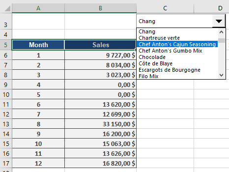
After selecting a product from the combo box, you want to display all sales for all countries that occurred within the year. Open a new worksheet and click on an empty cell. To test the GETPIVOTDATA() function, enter an equal sign (=) in the selected cell and then click any cell within the PivotTable you just created.
The GETPIVOTDATA() function will be applied automatically (see Figure below).

If you confirm the selected cell (cell B11 in the figure) by pressing the Enter key, the value $21,890 will appear in the worksheet (see Figure below).

Here are the arguments for the GETPIVOTDATA() function in this example: =GETPIVOTDATA(« Sales »,’Pivot from raw data’!$A$6, »Date »,1, »Product », »Camembert Pierrot »)
- « Sales »: This is the required data_field containing the data to be retrieved—in this case, the sales.
- ‘Pivot from original data’!$A$6: This is the pivot_table reference to cell A6 (or a cell range) within the PivotTable that contains the data you want to retrieve.
- « Date »,1: This is the first field1, item1 pair. « Date » is the field name, and 1 indicates January, meaning the sales for January are returned. 2 would indicate February, and so on.
- « Product », « Chai »: This is the first field2, item2 pair. « Product » is the field name, and « Chai » is the item name, meaning the sales for the product « Chai » are returned.
After familiarizing yourself with the GETPIVOTDATA() function, you decide to create a sales overview. Copy all item names from your original data list and paste them into the new worksheet (see Figure below).

Next, add a combo box to enable product selection from this list. If the « Developer » tab isn’t displayed, you’ll need to activate it.To add a combination field in Excel, right-click the menu bar and select « Form » to activate the « Form » toolbar. From the « Form » toolbar, drag a combination field onto the worksheet and open its properties. For « Input Range, » select the copied item names, and for « Cell Link, » assign an empty cell to the form.
When you click the arrow in the combo box, all item names will be available. In this example, the cell link is cell A2, and as a selection is made, the position of the selected entry in the list is displayed in this cell (see Figure below).
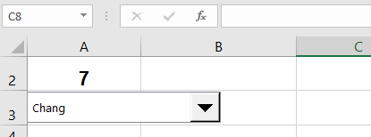
By using the INDEX() function, you can display the text value associated with the selection rather than just its position number. Click any empty cell in the worksheet and specify the arguments for the INDEX() function (see Figure below).
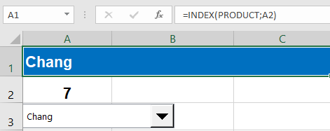
The following arguments are specified for the INDEX() function:
- array: This is the list of product names.
- row: A2 indicates the row or cell position to be returned.
- column: This argument doesn’t need to be specified because the row argument is used.
No matter which product you select in the combo box, the selection will be displayed as a label in cell A1.
To display the sales for each month, create a table with two columns: « Month » and « Sales. » Enter numbers 1 through 12 in the « Month » column, and then click the sales cell for month 1 (January). Enter an equal sign in this cell and click a cell under « January » in the PivotTable. Press the Enter key to confirm.
The Figure below shows the first entry in the sales cell for January.
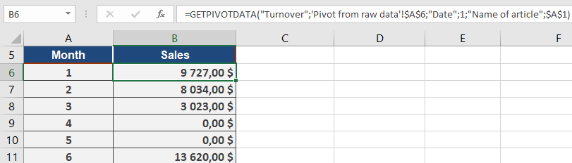
Now, you only need to modify the formula for the GETPIVOTDATA() function. The automatically generated formula displays the sales for January for the product « Alice Mutton. » Replace this with a reference to cell A1 to dynamically display the January sales for whatever product is selected in the combo box (see Figure below).

Finally, drag the formula in cell B6 down to the month of December to get the sales for all months, depending on the product selected in the combo box. The GETPIVOTDATA() function enables you to create neatly arranged summary tables.