This function searches for a value in the top row of a table or array and returns a corresponding value from the specified row.
Syntax:
HLOOKUP(lookup_value; table_array; row_index_num; [range_lookup])
Arguments:
- lookup_value (optional): The value to search for (text, number, or logical value).
- table_array (required): A cell range or array constant (enclosed in braces {}).
- row_index_num (required): A positive integer indicating which row to return (must not exceed the table’s rows).
- range_lookup (optional):
- FALSE → Searches for an exact match.
- TRUE or omitted → Finds the nearest match (≤ lookup_value).
Background:
- Exact Match (range_lookup = FALSE):
- Searches the top row for an exact match of lookup_value.
- Returns #N/A if no match is found.
- No sorting required.
- Approximate Match (range_lookup = TRUE or omitted):
- Returns an exact match if found; otherwise, the largest value ≤ lookup_value.
- Requires the top row to be sorted in ascending order.
Example:
A bus timetable requires finding minutes based on a stop (column) and time (row) as seen in the table below.
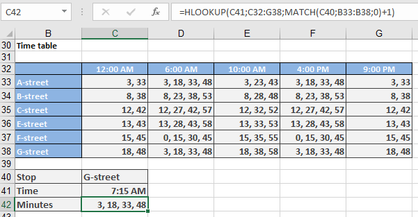
Since HLOOKUP() alone cannot handle row selection dynamically, combine it with MATCH():
=HLOOKUP(C41; C32:G38; MATCH(C40; B33:B38; 0) + 1)
- MATCH(C40; B33:B38; 0): Finds the stop (C40) in the first column.
- +1: Adjusts for the header row in table_array.