How to Use the IFERROR Function in Excel

The IFERROR function is used to return a custom result when a formula produces an error. It provides a simple way to handle errors without complex nested IF statements.

The IFERROR function uses the following syntax:

=IFERROR(value; value_if_error) 

Arguments:

• Value (Required): The formula or expression to be checked for errors
• Value_if_error (Required): The result to return if an error is detected

USING THE IFERROR FUNCTION

Using the table below, we’ll apply the IFERROR function to replace errors with the message « invalid data »:

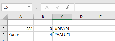
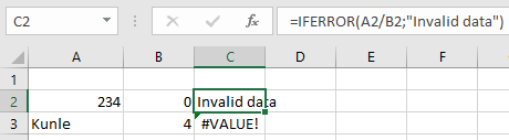
To correct the error in cell C2:

1. Select an empty cell
2. Enter the formula:

=IFERROR(A2/B2; « invalid data ») 

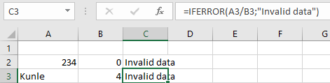
To correct the error in cell C3:

1. Select an empty cell
2. Enter the formula:

=IFERROR(A3/B3; « invalid data ») 

IMPORTANT NOTES ABOUT THE IFERROR FUNCTION

• If either value or value_if_error refers to an empty cell, IFERROR treats it as an empty string («  »)
• When applied to an array formula, IFERROR returns an array of results for each cell in the specified range
• Common errors handled by IFERROR include:
  • #N/A
  • #VALUE!
  • #REF!
  • #DIV/0!
  • #NUM!
  • #NAME?
  • #NULL!

The IFERROR function simplifies error handling in formulas while maintaining spreadsheet clarity and efficiency.