How to use the INDEX function in Excel

The INDEX function returns a value or reference from within a table or range based on specified row and column positions. This function is commonly used with MATCH and can serve as an alternative to VLOOKUP. The INDEX function has two formats:

1. Array Format
2. Reference Format

THE ARRAY FORMAT OF THE INDEX FUNCTION

The array format returns the value of a specific cell or range of cells within an array.

Syntax:

=INDEX(array; row_num; [col_num])

Arguments:

• array (Required):
  The range of cells to search within.
• row_num (Required):
  The row position in the array to return.
  • If set to 0 or omitted, returns all rows in the array.
• col_num (Optional):
  The column position in the array to return.
  • If set to 0 or omitted, returns all columns in the array.

USING THE ARRAY FORMAT OF THE INDEX FUNCTION

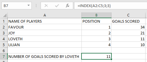
Example: Find Goals Scored by LOVETH

Given the following table (range A2:C5):

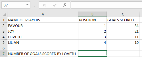
Steps to find Loveth’s goals (row 3, column 3):

1. Select an empty cell.
2. Enter the formula:

=INDEX(A2:C5; 3; 3)

1. Press Enter → Returns 11 (Loveth’s goals).