Calculates the y-intercept of the linear regression line fitted to a dataset. This is the point where the regression line crosses the y-axis (i.e., the predicted value of y when x = 0).
Syntax:
INTERCEPT(known_y’s; known_x’s)
Arguments
| Argument | Required? | Description |
| known_y’s | Yes | Dependent variable (response data). Must be a single row/column. |
| known_x’s | Yes | Independent variable (predictor data). Must match dimensions of known_y’s. |
Error Handling:
- Returns #N/A if:
- known_y’s and known_x’s have unequal lengths.
- Either argument is empty.
Background
Regression Analysis Context:
- Models the linear relationship between dependent (y) and independent (x) variables.
- The regression line minimizes the sum of squared deviations (least squares method).
Equation of the Line:
y=mx+b
Where:
- b= y-intercept (calculated by INTERCEPT()).
- m = slope (calculated by SLOPE()).
Intercept Formula:
b=yˉ−mxˉ
- yˉ: Mean of known_y’s.
- xˉ: Mean of known_x’s.
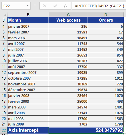
Example: Website Traffic Analysis
Scenario:
A company analyzes if orders (y) depend on website visits (x) (Jan 2007–Jun 2008).
Step 1: Calculate Intercept
=INTERCEPT(orders_range ; visits_range)
Result: 524.05 (see Figure below).
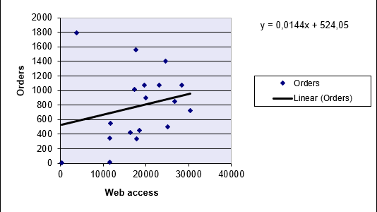
Step 2: Interpret Results
- The intercept (b = 524.05) implies:
- If there are zero visits, the model predicts 524 orders (theoretical baseline).
- Combined with the slope (m), it defines the regression line equation.
Visualization:
- A scatter plot with a trendline shows the intercept at y = 524.05 (Figure below).
Key Notes
- Usage with SLOPE():
- Use both functions to fully define the regression line:
y = SLOPE(y’s, x’s) * x + INTERCEPT(y’s, x’s)
- Assumptions:
- Linear relationship between x and y.
- Homoscedasticity (constant variance of residuals).
- Practical Applications:
- Forecasting sales based on advertising spend.
- Predicting exam scores from study hours.