
Searches for a specified value (lookup_value) within a row, column, or array and returns its relative position (not the value itself).
Syntax:
MATCH(lookup_value; lookup_array; [match_type])
Arguments:
| Argument | Required? | Description |
| lookup_value | Yes | The value to search for (text, number, or logical). Supports wildcards (*, ?) if match_type = 0. |
| lookup_array | Yes | A single row or column range or array to search. |
| match_type | No | Determines the match behavior: |
- 1 (default): Finds the largest value ≤ lookup_value (requires ascending order).
- 0: Finds the exact match (order irrelevant).
- -1: Finds the smallest value ≥ lookup_value (requires descending order). |
Key Rules & Background:
- Sorting Requirements:
- match_type = 1 → Data must be ascending (numbers → text → FALSE/TRUE).
- match_type = -1 → Data must be descending.
- match_type = 0 → No sorting needed (exact match).
- Wildcards (*, ?):
- Only work with match_type = 0.
- * = any sequence of characters.
- ? = any single character.
- Case Sensitivity:
- Not case-sensitive (e.g., « APPLE » = « apple »).
- Errors:
- #N/A → Value not found or invalid match_type for data.
Examples
The following examples show how this function is used.With the MATCH() function, you can quickly search multiple columns. Assume that you have a price list for clothing as seen below;
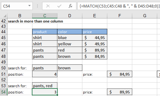
You can determine the position of the yellow shirt with the formula
{=MATCH(C50 & D50;C45:C48 & D45:D48;0)}
Because this is an array formula, you have to press Ctrl+Shift+Enter after entering the formula. The & links elements in the lookup_value and combines the two search columns into one column.
The INDEX() function returns the price:
=INDEX(E45:E48,C51)
Of course, you can combine both formulas into a single formula:
{=INDEX(E45:E48;MATCH(C50 & D50;C45:C48 & D45:D48;0))}
To enter the search criteria in a single row (C53 in Figure 9-9), use the following formula:
{=MATCH(C53;C45:C48 & « ; » & D45:D48;0)}
This is also an array formula. The search columns are now combined.
You can use the placeholders to find the elements even if you know only part of their names. If you enter pa in C58 and re in D58, the formula
{=MATCH(« * » & C58 & « * » & D58 & « * »;C45:C48 & D45:D48;0)}
finds the row containing the red pants.
Cross tabulations (the simplest form of PivotTable) are often used. These include tables such as time tables, distances between cities, and rate tables. Assume that you have a phone rate comparison table that tells you who the cheapest provider is at certain times of the day. As shows an example below.
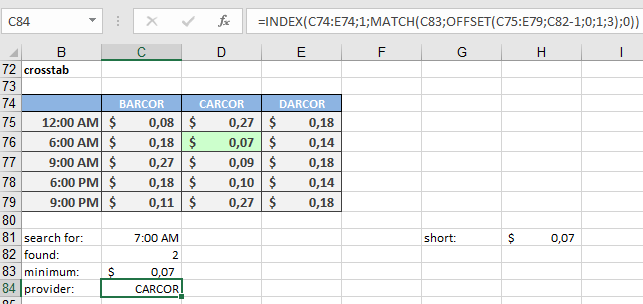
Looking for a time in the left column is a job for MATCH(). But what column contains the result? Use the MATCH() function to find the row, and
the MIN() and OFFSET() functions to find the cheapest rate. Here is the MATCH() function:
=MATCH(C81;B75:B79;1)
And here are the MIN() and the OFFSET() functions:
=MIN(OFFSET(C75:E79;C82-1;0;1;3))
You can combine both formulas into one. Thus, the following formula locates the provider who offers the cheapest rate:
=INDEX(C74:E74;1;MATCH(C83;OFFSET(C75:E79;C82-1;0;1;3);0))
Comparison with Other Functions:
| Feature | MATCH() | VLOOKUP()/HLOOKUP() | LOOKUP() |
| Returns | Position | Value | Value |
| Exact Match | Yes (with 0) | Yes (with FALSE) | No |
| Flexibility | High (works with INDEX) | Moderate | Low |
Pro Tips:
- Combine with INDEX() for dynamic lookups (superior to VLOOKUP).
- Use match_type = 0 for unsorted data or wildcard searches.
- Avoid #N/A with IFERROR():
=IFERROR(MATCH(…), « Not Found »)