The MATCH function is used to search for a specified value within a range of cells and returns the relative position of that value within the range.
Syntax:
=MATCH(lookup_value; lookup_array; [match_type])
Arguments:
- lookup_value (Required):
- The value you want to find within the lookup_array.
- lookup_array (Required):
- The range of cells being searched.
- match_type (Optional):
- Specifies how Excel matches the lookup_value with values in the lookup_array.
| match_type | Behavior |
| 1 or omitted | Finds the largest value ≤ lookup_value. Requires lookup_array to be sorted in ascending order. |
| 0 | Finds the first exact match. Does not require sorting. |
| -1 | Finds the smallest value ≥ lookup_value. Requires lookup_array to be sorted in descending order. |
USING THE MATCH FUNCTION
Example: Find the Position of « Apple »
Given the following table:
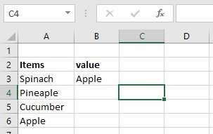
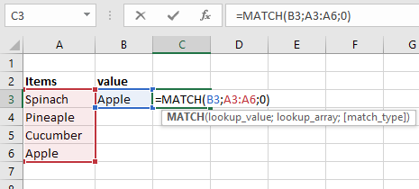
- Select an empty cell and enter
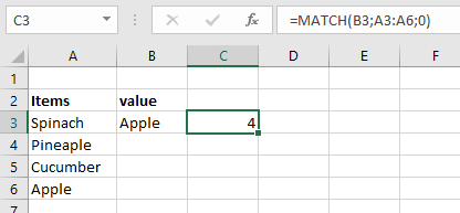
=MATCH(B3; A3:A6; 0)
(Where B3 contains « Apple »)
- Press Enter → Returns 4 (Apple is the 4th item in the range).
NOTES & ERRORS
- Case-Insensitive: Does not distinguish uppercase/lowercase.
- #N/A Error: Occurs if no match is found.
- Wildcards Supported: Use * (any sequence) or ? (single character) for partial matches.
- Exact vs. Approximate: Use match_type=0 for exact matches; 1 or -1 for approximate (requires sorted data).