This function calculates the net present value of future period surpluses (cash flows) of an investment based on a given discount rate.
Syntax
NPV(Rate; Value1; Value2; …)
Arguments
- Rate (required) – The discount rate supplied by the investor.
- Value1, Value2, … (required) – The (actual and expected) surpluses from disbursements and deposits, listed in a continuous column. Each value represents the end of a period (typically one year) in ascending order without gaps. Negative surpluses are indicated with a minus sign.
If the cells in the Value argument contain non-numeric data or are empty, Excel treats them as if they do not exist. This also applies if cell references in the argument point to such cells.
Background
Dynamic investment appraisal methods rely on estimated and projected deposits and disbursements and their yields, unlike static methods, which focus on costs and earnings. Both cash inflows and outflows are evaluated using a uniform discount rate derived from the investor’s experience. The sum of all discounted period surpluses is called the net present value (NPV).
An investment is considered financially viable if the NPV is non-negative, meaning the invested capital plus the expected yield is recovered.
The first value in the NPV() function represents the end of the first period. The net present value of an investment is determined by subtracting the initial disbursement (at the start of the first period) from the result of NPV().
Example
When reviewing the following examples, compare them to the explanations for IRR() and its related examples.
Investment in Material Assets
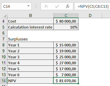
The purchase cost of a machine is $80,000.00. The expected annual surpluses (deposits minus disbursements) are estimated as shown in Table 1.
Table 1. Estimated Annual Surpluses from Machine Usage
| Year | Surplus (in $) |
| 1 | 15,000 |
| 2 | 19,000 |
| 3 | 25,000 |
| 4 | 27,000 |
| 5 | 17,000 |
| 6 | 7,000 |
Is the investment economically sound if a discount rate of 10% p.a. is applied?
To answer this, enter the purchase cost in the first cell and list the surpluses from Table 1 in a continuous column. Using NPV() returns approximately $81,070, slightly exceeding the purchase cost. Thus, the yield is likely marginally better than the expected rate.
Note: Decimal precision may not be critical when dealing with real investments where future surpluses are estimates.
Financial Investment
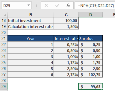
German federal savings bonds (Type A) with the terms as of August 30, 2010 (Table 2) may appear to offer a total yield of around 1.5% at first glance.
Table 2. Terms for Federal Savings Bonds
| Duration Year | Nominal Interest |
| 2010/2011 | 0.25% |
| 2011/2012 | 0.50% |
| 2012/2013 | 1.00% |
| 2013/2014 | 1.75% |
| 2014/2015 | 2.50% |
| 2015/2016 | 2.75% |
Sample calculations (available in the function’s example files) show that the net present value for a $100.00 investment is only $99.63. Therefore, investing at this expected yield is not advisable.