Returns the Pearson correlation coefficient (*r*), a dimensionless value between –1.0 and 1.0 that quantifies the linear relationship between two datasets.
Syntax:
PEARSON(array1; array2)
Arguments:
- array1 (required) – Independent variable (*x*) values.
- array2 (required) – Dependent variable (*y*) values.
Background:
- Interpretation of *r*:
- +1: Perfect positive linear correlation.
- –1: Perfect negative linear correlation.
- 0: No linear correlation.
- Limitations:
- Only measures linear relationships (ignores nonlinear patterns).
- Does not imply causation.
- Formula:
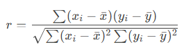
Where xˉ and yˉ are the means of array1 and array2.
Example:
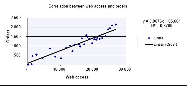
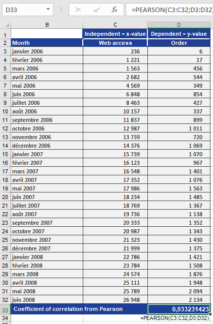
A software company analyzes the relationship between website visits (x) and online orders (y).
- Scatter Plot (Figure below): Visual linear trend suggests correlation.
- Calculation:
=PEARSON(B2:B100, C2:C100) // Returns r = 0.933
Result (Figure below):
-
- r=0.933r=0.933 → Strong positive correlation.
- Interpretation: Increased website visits closely align with increased orders.
Key Notes:
- High *r* ≠ Causation: Confounding factors (e.g., marketing campaigns) may influence results.
- Always visualize data (e.g., scatter plots) to validate linearity.