
Its calculates the present value of an investment based on a constant interest rate and a series of future payments (annuities) and/or a lump sum.
Syntax
PV(Rate; Nper; [Pmt]; [Fv]; [Type])
Arguments
| Argument | Requirement | Description | Financial Meaning |
| Rate | Required | Interest rate per period | Cost of capital/discount rate |
| Nper | Required | Total number of periods | Investment/loan term |
| [Pmt] | Conditionally Required | Payment per period | Annuity amount |
| [Fv] | Optional | Future value | Target balance/residual value |
| [Type] | Optional | Payment timing: 0 = end period (default) 1 = beginning period |
Cash flow timing |
Note: Either Pmt or Fv must be provided.
Financial Model
Implements the time value of money principle:
PV + Σ[Pmt/(1+Rate)^k] + Fv/(1+Rate)^Nper = 0
where k ranges from 1 to Nper (adjusted for Type).
Key Applications
- Lump Sum Investments (Retirement Planning)
=PV(Rate, Nper,, Fv)
- Annuity Valuation (Pension Planning)
=PV(Rate, Nper, Pmt)
- Loan Capacity (Mortgage Underwriting)
=PV(Rate, Nper, -Pmt)
Examples
- Retirement Savings Verification
Scenario:
$10,000 invested for 15 years at 5% p.a. targeting $25,000.
Calculation:
=PV(5%, 15,, 25000)
Result: -$12,025.43
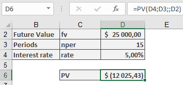
Interpretation: Requires $12,025 initial investment to reach target (current $10,000 insufficient).
- Mortgage Qualification
Scenario:
$1,000 monthly payment capacity for 30 years at 5.5% p.a.
Calculation:
=PV(5.5%/12, 30*12, -1000)
Result: $176,121.76
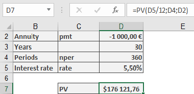
Interpretation: Maximum loan amount at given terms.
Important Notes
- Sign Convention:
- Positive results = Cash inflows
- Negative results = Cash outflows
- Compounding Assumptions:
- For monthly payments, divide annual rate by 12
- For quarterly payments, divide annual rate by 4
- Precision Tip:
For loan amortization schedules, combine with ROUND():
=ROUND(PV(…), 2)