How to Use the REFERENCE FORMAT OF THE INDEX Function in Excel

The reference format of the INDEX function returns a cell reference at the intersection of specified row and column numbers within one or more ranges.

Syntax:

=INDEX(reference; row_num; [column_num]; [area_num])

Arguments:

• reference (Required):
  One or more cell ranges. Multiple ranges must be separated by commas and enclosed in parentheses (e.g., (A1:B2;D5:E6)).
• row_num (Required):
  The row position within the reference.
  • If 0, returns a reference to all rows in the range.
• column_num (Optional):
  The column position within the reference.
  • If 0, returns a reference to all columns in the range.
• area_num (Optional):
  Specifies which range to use when multiple ranges are provided in reference.
  • Defaults to 1 (first range) if omitted.

USING THE REFERENCE FORMAT OF THE INDEX FUNCTION

Example: Find the Price of Mango

Given the following table (range A2:C10):

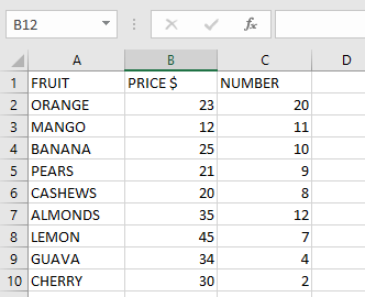
Steps to find Mango’s price (row 2, column 3, area 1):

1. Select an empty cell.
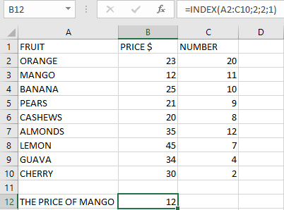
2. Enter the formula:

=INDEX((A2:C10); 2; 3; 1)

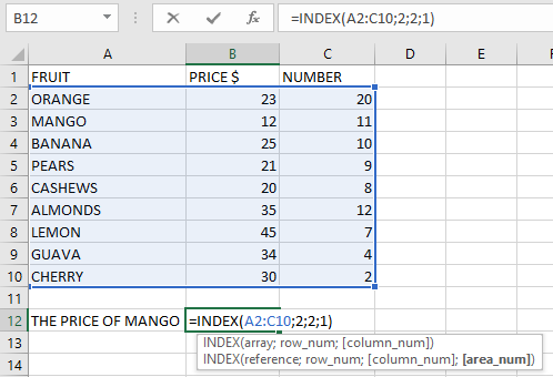
1. Press Enter → Returns 12 (Mango’s price).

NOTES & ERROR HANDLING

1. Return Behavior:
   • Returns the value at the row/column intersection when both row_num and column_num are specified.
   • Returns an array of values if either row_num or column_num is 0.
2. Common Errors:
   • #VALUE!: Occurs if row_num, column_num, or area_num is non-numeric.
   • #REF!: Occurs when:
     • row_num exceeds the range’s row count.
     • column_num exceeds the range’s column count.
     • area_num exceeds the number of provided ranges.
3. Multi-Range Example:

=INDEX((A1:B2;D5:E6); 1; 2; 2)

Returns the value from row 1, column 2 of the second range (D5:E6).