Returns the row number of a specified cell or range. If no argument is provided, it returns the row number of the cell containing the formula.
Syntax:
ROW([reference])
Arguments:
| Argument | Required? | Description |
| reference | No | A cell or range (e.g., A1, B2:D5). If omitted, defaults to the formula’s cell. |
Key Behavior:
- Single Cell Reference:
- =ROW(C10) → Returns 10.
- Range Reference:
- =ROW(B2:D5) → Returns an array of row numbers {2;3;4;5} (requires Ctrl+Shift+Enter in older Excel).
- Omitting Reference:
- If entered in cell F7, =ROW() → Returns 7.
Examples:
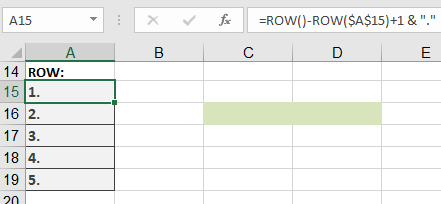
- Generate Consecutive Numbers
- Formula in A15:
=ROW() – ROW($A$15) + 1 & « . »
-
- Result in A15: 1.
- Copied down: 2., 3., etc.
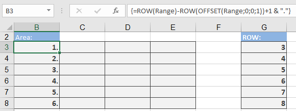
- Dynamic Numbering in a Named Range
- Array Formula (Ctrl+Shift+Enter in legacy Excel):
{=ROW(Range) – ROW(OFFSET(Range, 0, 0, 1)) + 1 & « . »}
-
- How It Works:
- ROW(Range) → Array of row numbers in the range.
- ROW(OFFSET(…; 1)) → Gets the first row of the range.
- Subtracting adjusts numbering to start at 1.
- How It Works:
- Extract Row Number from a Cell
- Formula:
=ROW(INDEX(5:5; 1; 1))
-
- Result: 5 (returns the row number of row 5).
Common Errors & Fixes:
| Error | Cause | Solution |
| #VALUE! | Non-reference argument (e.g., ROW(« text »)). | Use a valid cell/range reference. |
| #N/A | Output range larger than input (array formulas). | Match output size to input. |
Advanced Uses:
- Conditional Formatting (Highlight Every 3rd Row)
- Rule Formula:
=MOD(ROW(); 3) = 0
- Dynamic Sum Based on Row Position
- Formula:
=SUM(A1:INDEX(A:A; ROW() – 1))
-
- Sums all cells above the formula’s row.
- Find Last Used Row in Column A
- Formula:
=MAX(ROW(A:A)*(A:A<> » »))
-
- Note: Enter with Ctrl+Shift+Enter in legacy Excel.
Comparison with ROWS():
| Function | Returns | Example |
| ROW() | Row number of a cell. | =ROW(A3) → 3 |
| ROWS() | Count of rows in a range. | =ROWS(A1:A10) → 10 |