Its returns the sign of a number as:
- 1 if the number is positive
- 0 if the number is zero
- -1 if the number is negative
Syntax:
SIGN(number)
Argument:
| Argument | Description |
| number (required) | Any real number. |
Background:
- Positive numbers are > 0 (plus sign + optional).
- Negative numbers are < 0 (minus sign – required).
- Zero is neutral (neither positive nor negative).
Examples:
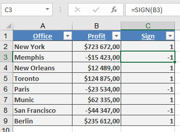
- Filtering Negative Revenues
Scenario: Identify subsidiaries with losses in a sales list.
Step 1: Add a column with SIGN() to flag revenue signs:
=SIGN(B2) // Returns -1 for losses, 1 for profits
Step 2: Calculate total losses (negative values):
{=SUM(IF(SIGN(B2:B9)=-1, B2:B9))} // Array formula (Ctrl+Shift+Enter)
Step 3: Calculate total profits (positive values):
{=SUM(IF(SIGN(B2:B9)=1, B2:B9))} // Array formula (Ctrl+Shift+Enter)
Additional Use Cases:
- Conditional Formatting: Highlight negative values.
- Data Validation: Restrict inputs to positive numbers.
Key Notes:
- Simple but powerful for data analysis and validation.
- Often combined with IF(), SUMIF(), or array formulas.