How to use the SUMIF function in Excel

The SUMIF function calculates the total of cells that meet specific conditions. These conditions can be based on dates, numbers, or text values. The function supports logical operators (<, >, =, etc.) and wildcard characters (*, ?).

The SUMIF function uses these arguments:
=SUMIF(range; criteria; [sum_range])

Range (Required):
This is the group of cells that will be checked against your criteria.

Criteria (Required):
This determines which cells to include in the sum. You can use:

• Numbers (like 10, 0.5, or 12:00)
• Text (such as « January », « North »)
• Expressions (for example, « >100 » or « <=50 »)

Sum_range (Optional):
These are the actual cells to add together. If you leave this out, Excel will sum the cells in your range instead.

HOW TO USE SUMIF FUNCTION

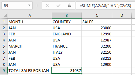
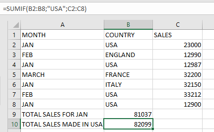
Let’s see how this works with two practical examples: calculating January sales using the table below;

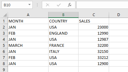
Example 1: Calculate January Sales

1. Click on an empty cell
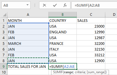
2. Type the formula:
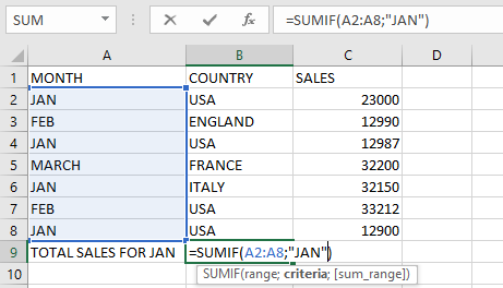
   =SUMIF(A2:A8; « Jan »; C2:C8)
   • A2:A8 contains month names

1. • « Jan » is our condition

1. • C2:C8 has the sales numbers

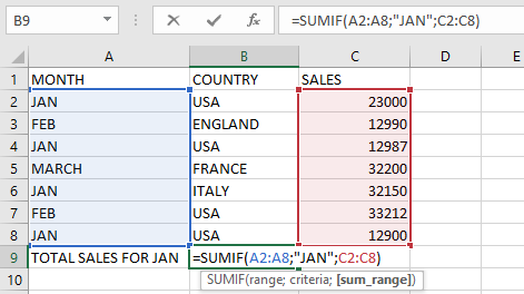
1. Press Enter to see the result: 81037

Example 2: Calculate USA Sales

1. Select an empty cell
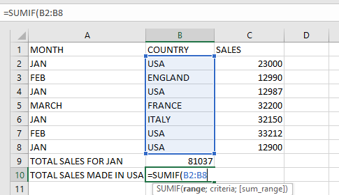
2. Enter the formula:
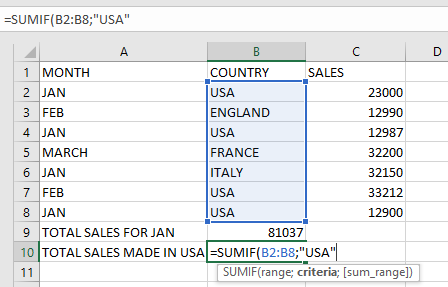
   =SUMIF(B2:B8; « USA »; C2:C8)
   • B2:B8 lists countries

1. • « USA » is our criteria

1. • C2:C8 contains the sales figures

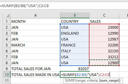
1. Hit Enter to view the total USA sales

IMPORTANT NOTES

1. If you see #VALUE!, your criteria might be too long (over 255 characters)
2. When you don’t specify sum_range, Excel sums the cells in your range
3. Always put text criteria in « double quotes »
4. Wildcards work in SUMIF:

• matches multiple characters (e.g., « A* » finds « Apple »)

1. • ? matches one character (e.g., « J?n » finds « Jan » or « Jun »)