This function searches for a value in the leftmost column of a table and returns a value from the same row in a specified column. The range_lookup argument determines whether an exact or approximate match is required.
Syntax
VLOOKUP(lookup_value; table_array; col_index_num;[range_lookup])
Arguments
- lookup_value (required)
Can be text, a number, or a logical value. This is the value to search for in the first column of the table. - table_array (required)
A reference to a range of cells or an array constant (numbers and text must be enclosed in braces {}). - col_index_num (required)
Must be a positive integer indicating the column number from which to return the value. The leftmost column is 1. - range_lookup (optional)
A logical value:- TRUE (or omitted): Finds the closest match (approximate).
- FALSE: Requires an exact match.
Background
- If range_lookup is FALSE, VLOOKUP() searches for an exact match in the first column. If none is found, it returns #N/A. The table does not need to be sorted.
- If range_lookup is TRUE or omitted, the function returns:
- An exact match if one exists.
- Otherwise, the largest value less than lookup_value.
- Note: In this case, the table must be sorted in ascending order to ensure correct results.
Examples
The following examples demonstrate how to use VLOOKUP().
Combining with Other Functions
The INDEX() function can be used with VLOOKUP() to find exact matches.
- VLOOKUP() only retrieves values to the right of the search column.
- For more flexible searches across a table, use INDEX() and MATCH().
Example Scenario:
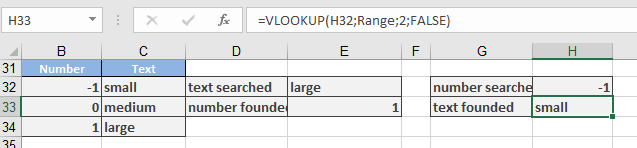
Assume a table (Range = B32:C34) assigns numbers to text (e.g., -1 = small).
- Finding text from a number:
=VLOOKUP(-1; Range; 2; FALSE)
Returns « small ».
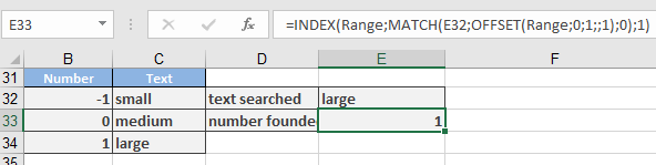
- Finding a number from text (inverse lookup):
=INDEX(Range; MATCH(F32; OFFSET(Range; 0; 1; ; 1); 0); 1)
-
- OFFSET() shifts the search to the second column.
- MATCH() finds the row containing the value in F32.
- INDEX() retrieves the corresponding value from column 1.