Implement Advanced Data Correlation Analysis with Excel VBA

Overview of the Task:

The goal is to create an Excel VBA code that can analyze and compute correlations between multiple data sets. This will involve calculating the Pearson correlation coefficient, which quantifies the linear relationship between two variables. The code will also include an option to analyze correlations for multiple data columns, generate a correlation matrix, and visualize the results using a heatmap.

Steps involved in the implementation:

1. Calculate Pearson Correlation Coefficient:
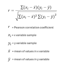
   • Pearson’s correlation coefficient (r) measures the strength and direction of a linear relationship between two variables. The formula for the Pearson correlation is:

1. Generate a Correlation Matrix:
   • If you have multiple data columns, the correlation matrix will show the Pearson correlation for every pair of columns.
2. Create a Heatmap for Visualization:
   • A correlation heatmap will help visualize the strength and direction of correlations between variables.

VBA Code for Correlation Analysis:

Option Explicit
' This function calculates the Pearson correlation between two arrays of data.
Function PearsonCorrelation(arrX As Range, arrY As Range) As Double
    Dim i As Long
    Dim n As Long
    Dim sumX As Double, sumY As Double
    Dim sumXY As Double, sumX2 As Double, sumY2 As Double
    Dim correlation As Double
    n = arrX.Count
    If n <> arrY.Count Then
        MsgBox "Ranges must have the same number of rows.", vbCritical
        Exit Function
    End If
    ' Initializing sums
    sumX = 0
    sumY = 0
    sumXY = 0
    sumX2 = 0
    sumY2 = 0
    ' Loop through each value and compute the sums required for Pearson's formula
    For i = 1 To n
        sumX = sumX + arrX.Cells(i, 1).Value
        sumY = sumY + arrY.Cells(i, 1).Value
        sumXY = sumXY + arrX.Cells(i, 1).Value * arrY.Cells(i, 1).Value
        sumX2 = sumX2 + arrX.Cells(i, 1).Value ^ 2
        sumY2 = sumY2 + arrY.Cells(i, 1).Value ^ 2
    Next i
    ' Pearson Correlation formula
    correlation = (n * sumXY - sumX * sumY) / _
                  Sqr((n * sumX2 - sumX ^ 2) * (n * sumY2 - sumY ^ 2))
    PearsonCorrelation = correlation
End Function

' This subroutine calculates the correlation matrix for a range of columns.
Sub CorrelationMatrixAnalysis()
    Dim dataRange As Range
    Dim i As Long, j As Long
    Dim numColumns As Long
    Dim correlationResult As Double
    Dim matrixRange As Range   
    ' Specify the data range (assume data starts in cell A1)
    Set dataRange = Range("A1").CurrentRegion
    numColumns = dataRange.Columns.Count
    ' Output header for the correlation matrix
    With dataRange.Worksheet
        ' Set header for correlation matrix
        Set matrixRange = .Range("G1").Resize(numColumns, numColumns)
        matrixRange.Cells(1, 1).Value = "Correlation Matrix"       
        ' Loop through each combination of columns to calculate Pearson correlation
        For i = 1 To numColumns
            For j = 1 To numColumns
                ' Skip diagonal elements (correlation of a column with itself is always 1)
                If i = j Then
                    matrixRange.Cells(i + 1, j + 1).Value = 1
                Else
                    ' Calculate Pearson correlation between columns i and j
                    correlationResult = PearsonCorrelation(dataRange.Columns(i), dataRange.Columns(j))
                    matrixRange.Cells(i + 1, j + 1).Value = correlationResult
                End If
            Next j
        Next i
    End With
    MsgBox "Correlation Matrix Calculated Successfully"
End Sub

' This subroutine creates a color-coded heatmap for the correlation matrix.
Sub CreateHeatmap()
    Dim matrixRange As Range
    Dim cell As Range
    Dim correlationValue As Double
    Dim color As Long   
    ' Set the range for the correlation matrix (output from CorrelationMatrixAnalysis)
    Set matrixRange = Range("G2").CurrentRegion   
    ' Loop through each cell in the matrix and color based on correlation value
    For Each cell In matrixRange
        correlationValue = cell.Value       
        ' Apply colors based on correlation value
        If correlationValue > 0.8 Then
            color = RGB(0, 255, 0) ' Green for high positive correlation
        ElseIf correlationValue > 0.5 Then
            color = RGB(255, 255, 0) ' Yellow for moderate positive correlation
        ElseIf correlationValue < -0.8 Then
            color = RGB(255, 0, 0) ' Red for high negative correlation
        ElseIf correlationValue < -0.5 Then
            color = RGB(255, 165, 0) ' Orange for moderate negative correlation
        Else
            color = RGB(200, 200, 200) ' Gray for weak correlation
        End If       
        cell.Interior.Color = color
    Next cell
    MsgBox "Heatmap Created Successfully"
End Sub

Detailed Explanation of the Code:

1. PearsonCorrelation Function:
   • This function computes the Pearson correlation coefficient for two data ranges (arrays).
   • It checks if the data ranges have the same number of rows.
   • It calculates the required sums (sum of X, sum of Y, sum of XY, sum of X^2, and sum of Y^2).
   • It then uses these sums to compute the Pearson correlation using the Pearson correlation formula.
2. CorrelationMatrixAnalysis Subroutine:
   • This subroutine calculates the correlation matrix for a set of data columns.
   • The data range is assumed to start from cell A1 and covers all adjacent rows and columns.
   • The code loops through each pair of columns in the dataset, computes the correlation for each pair using the PearsonCorrelation function, and stores the result in a new range (starting at G1).
   • The diagonal elements (correlations of a column with itself) are set to 1, as the correlation of a variable with itself is always 1.
3. CreateHeatmap Subroutine:
   • This subroutine applies a color code to the correlation matrix based on the correlation values.
   • It uses green for strong positive correlations (greater than 0.8), red for strong negative correlations (less than -0.8), and various shades for other levels of correlation.
   • The heatmap provides a visual representation of the correlation strengths between data columns.

Usage:

1. Running the Analysis:
   • Open Excel and press ALT + F11 to open the VBA editor.
   • Insert a new module, and paste the code into it.
   • To run the analysis, press F5 while the CorrelationMatrixAnalysis or CreateHeatmap subroutine is selected.
2. Input Data:
   • The data should be organized in columns, where each column represents a different variable or dataset.
   • The code will compute the correlations between these variables.
3. Output:
   • The correlation matrix will be placed in a new range starting from cell G1.
   • The heatmap will color-code the matrix based on correlation strength.

Conclusion:

This advanced VBA code allows you to calculate and visualize correlations between multiple datasets in Excel. It is highly customizable, and you can extend it further by including other correlation types (e.g., Spearman’s rank correlation) or adding more visualization features. The heatmap is particularly useful for visually identifying strong relationships between variables.