Implement Advanced Inventory Management Algorithms with Excel VBA

I will walk you through both concepts step by step, including how to implement them in Excel VBA.

1. ABC Analysis

ABC Analysis is a method for classifying inventory into three categories (A, B, and C) based on their importance, typically using the annual consumption value.

Steps to implement ABC Analysis:

• Category A: These are the most important items, usually accounting for 70-80% of the value, but only a small percentage (10-20%) of the items.
• Category B: These items represent a moderate value, accounting for about 15-25% of the value, and 20-30% of the items.
• Category C: These are the least important, but usually make up a large percentage of the inventory in terms of volume (50-60% of items), yet only account for 5-10% of the value.

Steps to implement in VBA:

• Calculate the Annual Consumption Value for each item by multiplying the unit cost by the annual demand (usage).
• Sort items by Annual Consumption Value in descending order.
• Compute cumulative consumption percentage and classify items into A, B, or C based on their contribution to total value.

Excel VBA Code for ABC Analysis:

Sub ABCAnalysis()
    Dim ws As Worksheet
    Set ws = ThisWorkbook.Sheets("Inventory") ' Change to your sheet name
    Dim lastRow As Long
    lastRow = ws.Cells(ws.Rows.Count, "A").End(xlUp).Row ' Assuming data starts from row 2   
    ' Columns (Assumed): A=Item, B=Unit Cost, C=Annual Demand, D=Annual Consumption Value, E=ABC Category
    Dim totalConsumptionValue As Double
    totalConsumptionValue = Application.WorksheetFunction.Sum(ws.Range("D2:D" & lastRow)) ' Sum of Consumption Values   
    Dim cumulativeConsumptionValue As Double
    cumulativeConsumptionValue = 0   
    ' Step 1: Calculate Annual Consumption Value (Unit Cost * Annual Demand)
    Dim i As Long
    For i = 2 To lastRow
        ws.Cells(i, 4).Value = ws.Cells(i, 2).Value * ws.Cells(i, 3).Value ' Annual Consumption Value (Unit Cost * Annual Demand)
    Next i   
    ' Step 2: Sort the inventory by Annual Consumption Value (Column D) in descending order
    ws.Range("A1:E" & lastRow).Sort Key1:=ws.Range("D2:D" & lastRow), Order1:=xlDescending, Header:=xlYes   
    ' Step 3: Calculate cumulative percentage of the total consumption value
    For i = 2 To lastRow
        cumulativeConsumptionValue = cumulativeConsumptionValue + ws.Cells(i, 4).Value
        ws.Cells(i, 5).Value = cumulativeConsumptionValue / totalConsumptionValue * 100 ' Cumulative percentage       
        ' Step 4: Classify into A, B, or C based on cumulative percentage
        If ws.Cells(i, 5).Value <= 80 Then
            ws.Cells(i, 5).Value = "A"
        ElseIf ws.Cells(i, 5).Value <= 95 Then
            ws.Cells(i, 5).Value = "B"
        Else
            ws.Cells(i, 5).Value = "C"
        End If
    Next i   
    MsgBox "ABC Analysis Complete!"
End Sub

Explanation of ABC Analysis Code:

1. Item Classification:
   • Annual Consumption Value is calculated in column D by multiplying the unit cost (column B) by the annual demand (column C).
   • The data is sorted by the annual consumption value (column D), from highest to lowest.
   • The cumulative consumption percentage is calculated, which is the sum of the annual consumption value divided by the total consumption value.
   • The ABC classification is based on cumulative percentage:
     • A: Top 70-80% of the value.
     • B: Next 15-25% of the value.
     • C: The remaining 5-10% of the value.

2. Economic Order Quantity (EOQ)

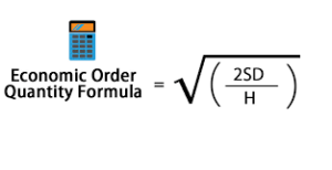
Steps to implement EOQ in VBA:

1. Define the parameters: Demand (D), Ordering cost (S), and Holding cost (H).
2. Calculate EOQ using the formula.
3. You can also calculate the total inventory cost, which is the sum of the ordering cost and holding cost.

Excel VBA Code for EOQ Calculation:

Sub EOQCalculation()
    Dim ws As Worksheet
    Set ws = ThisWorkbook.Sheets("Inventory") ' Change to your sheet name
    Dim lastRow As Long
    lastRow = ws.Cells(ws.Rows.Count, "A").End(xlUp).Row ' Assuming data starts from row 2   
    ' Columns (Assumed): A=Item, B=Annual Demand (D), C=Ordering Cost (S), D=Holding Cost (H), E=EOQ, F=Total Cost
    Dim EOQ As Double
    Dim orderingCost As Double, holdingCost As Double, demand As Double   
    Dim i As Long
    For i = 2 To lastRow
        ' Step 1: Get Demand, Ordering Cost, and Holding Cost
        demand = ws.Cells(i, 2).Value
        orderingCost = ws.Cells(i, 3).Value
        holdingCost = ws.Cells(i, 4).Value       
        ' Step 2: Calculate EOQ using the EOQ formula
        EOQ = Sqr((2 * demand * orderingCost) / holdingCost)       
        ' Step 3: Calculate Total Cost (Ordering Cost + Holding Cost)
        ws.Cells(i, 5).Value = EOQ ' Store EOQ in column E
        ws.Cells(i, 6).Value = (demand / EOQ) * orderingCost + (EOQ / 2) * holdingCost ' Total cost in column F
    Next i   
    MsgBox "EOQ Calculation Complete!"
End Sub

Explanation of EOQ Code:

1. Inputs:
   • Demand (D), Ordering Cost (S), and Holding Cost (H) are obtained from the spreadsheet for each item.
2. EOQ Calculation: The EOQ formula is implemented using Sqr((2 * D * S) / H), and the result is stored in column E.
3. Total Cost Calculation: The total inventory cost for each item is calculated as:
   • Ordering Cost: DEOQ×S\frac{D}{EOQ} \times S
   • Holding Cost: EOQ2×H\frac{EOQ}{2} \times H

Summary:

• The ABC Analysis helps in classifying inventory into three categories based on their importance, aiding in prioritizing items for inventory management.
• The EOQ model helps to calculate the optimal order quantity to minimize inventory costs, balancing between holding costs and ordering costs.

These two techniques are fundamental for effective inventory management and can be easily implemented in Excel VBA to automate the process.