The mean provides a measure of central tendency by considering all the actual values in a group. The median measures central tendency differently, providing the midpoint of a sorted group of values. The mode takes another approach: it tells you which of several values occurs most frequently. While the mean and median require certain calculations, a mode value can be found simply by counting how many times each value occurs.
For example, the mode of the dataset {1, 2, 2, 3, 4, 6} is 2. In Microsoft Excel, you can calculate the mode using the function of the same name: MODE. For our example dataset, the formula would be:
=MODE(B2:B10)
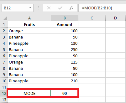
In situations where there are two or more modes in your dataset, the Excel MODE function will return the lowest mode.
Determining the Mode of Nominal Data Using Pivot Tables
However, the MODE() function does not work with nominal data. If you present it with a range that contains only text data such as names, MODE() will return the #N/A error. If one or more text values are included in a list of numerical values, MODE() simply ignores the text values.
In such cases, pivot tables can be a helpful alternative to find the mode. Here is a quick overview of the process:
- Prepare Your Data: Arrange your raw data in a list format in Excel. The field name in the first column (like A1) and the values in the cells below (like A2:A21). It’s better if all cells adjacent to the list are empty.
- Insert a Pivot Table:
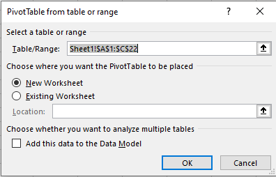
- Click on the Insert tab on the ribbon, then select Pivot Table in the Charts group.
- Excel will automatically populate the range in the Table/Range field if you selected a cell in your list before clicking Pivot Table.
- Configure Your Pivot Table:
- Place the field(s) you’re interested in into the Rows and Values areas of the PivotTable Field List.
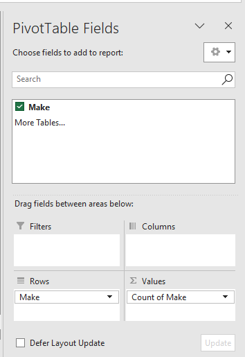
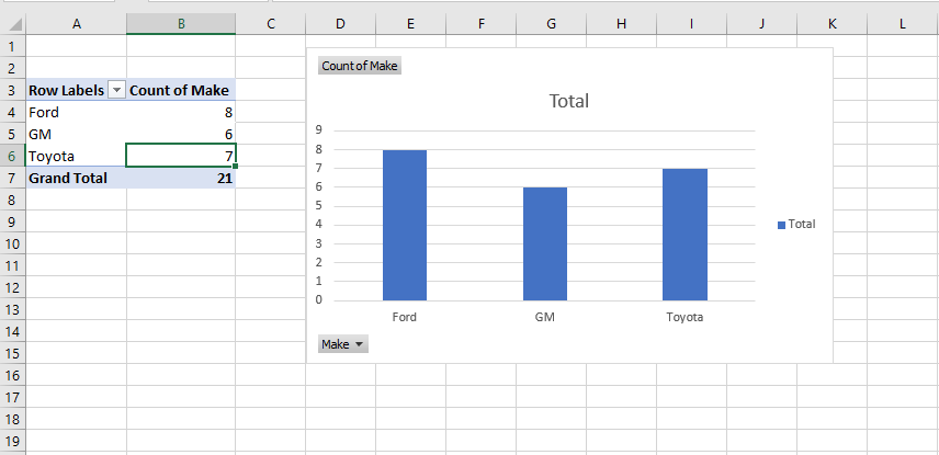
The PivotTable will now show the frequency distribution, where the mode is the value that occurs most often.
Comments on the Mode Analysis
- The mode is a very useful statistic when applied to categories such as political parties, popular brands, weekdays, and regions. Excel should have an integrated function for the mode of text values. While it doesn’t, the next section will show you how to write your own formula for the mode that works with both numerical and text values.
- When you only have a few distinct categories, consider creating a pivot table to show the count of each category. A pivot table that shows the count of instances of each category is an attractive way to present your data to an audience.
- Standard Excel charts don’t show the number of instances per category without prior work. You should count each category before creating the chart, which is the purpose of the PivotTable supporting the PivotChart. The PivotTable is simply a faster way to perform the analysis than manually creating a table for counting category membership and then building a standard Excel chart based on it.
- The mode is the only sensible measure of central tendency when working with nominal data such as category names. The median requires sorting things in some way: from shortest to longest, cheapest to most expensive, or slowest to fastest. In terms of scale types, you need at least an ordinal scale to get a median, and many categories are nominal, not ordinal. Variables represented by values like Ford, GM, and Toyota don’t have a meaningful mean or median.
Getting the Mode of Categories with a Formula
The MODE() function in Excel doesn’t work when you provide text values as arguments. Here’s a method to get the mode using a formula. This formula will tell you which text value appears most frequently in your dataset. You’ll also learn how to create a formula to count the number of instances of the existing mode.
If you don’t want to use a PivotChart to find the mode of a group of text values, you can find it using the following formula:
=INDEX(A2:A21, MODE(MATCH(A2:A21, A2:A21, 0)))
Assuming the text values are in A2:A21 (the range could occupy a single column like A2:A21 or a single row like A2:Z2, but it won’t work properly with a multi-column range like A2:Z21).
If you’re new to Excel, this formula may look confusing. I’ve structured it based on my long experience with Excel, and I still need to pause and think about it before I can explain why it returns the mode. So, don’t worry if it seems puzzling right now. Over time, it will become clearer, and for now, you can use it to get the modal value for any set of text values in a worksheet.
Formula breakdown:
- The MATCH() function returns the position in the array where each value first appears. The third argument of MATCH() is set to 0, meaning an exact match is required, and the array doesn’t need to be sorted. So, for every instance of Ford in the values array A2:A21, MATCH() returns 1; for every instance of Toyota, it returns 2; and for GM, it returns 4.
- The results of the MATCH() function are used as an argument for the MODE() function. In this example, MODE() evaluates 20 values: some equal 1, some equal 2, and others equal 4. MODE() returns the most frequent of these numbers.
- The result of MODE() is then used as the second argument for the INDEX() function. The first argument is the array to check. The second argument tells INDEX() how far to look in the array. Here, it looks at the first value, which is Ford. If GM had been the most frequent text value, MODE() would have returned 4, and INDEX() would have used that value to find GM in the array.
Using an Array Formula to Count the Values
Once you have the modal value (Ford in this example), you still want to know how many instances of this mode exist. This section describes how to create the array formula to count the instances.
For this, use the following formula:
=SUM(IF(A2:A21 = C1, 1, 0))
This is an array formula and must be entered using the special key combination Ctrl + Shift + Enter. You’ll know it’s an array formula if you see curly braces around it in the formula bar.
Formula breakdown:
- The A2:A21 = C1 part checks whether each value in the range A2:A21 equals the value in cell C1 (Ford in this example).
- This results in a TRUE or FALSE array.
- The IF() function then converts these values: TRUE becomes 1 and FALSE becomes 0.
- The SUM() function adds up all the 1s (the instances of the mode).
For example, if Ford is the mode, the formula will count how many times Ford appears in the range A2:A21.
Recap of the Array Formula
To summarize how the array formula counts values for the modal category Ford, consider the following:
- The goal is to count how many times Ford appears in the range A2:A21.
- The A2:A21 = C1 part creates a TRUE/FALSE array depending on whether each cell matches Ford.
- The IF() function turns TRUE into 1 and FALSE into 0.
- The SUM() function adds up the 1s and 0s, giving the count of instances of Ford.
This array formula efficiently counts occurrences of the modal value in a given range.