Finance

Charts

Statistics

Macros

Search

Normal distribution in Excel

A normal distribution, also known as a Gaussian distribution, is a type of probability distribution in which the values of a random variable are distributed symmetrically around the central tendency—typically the mean. In this distribution, data points are equally spread on both sides of the mean, creating a characteristic bell-shaped curve when graphed.

This curve illustrates that most values cluster around the mean, while the frequency of extreme values (either very high or very low) decreases progressively as one moves away from the center. The peak of the curve corresponds to the mean, median, and mode, which are all equal in a perfect normal distribution.

Furthermore, the empirical rule (or 68-95-99.7 rule) applies to normal distributions. According to this rule:

  • Approximately 68% of the data values fall within one standard deviation from the mean.

  • Around 95% lie within two standard deviations.

  • And about 99.7% of the data is contained within three standard deviations of the mean.

This predictable pattern makes the normal distribution a fundamental concept in statistics, widely used in natural and social sciences to model real-world phenomena.

Explanation of the Normal Distribution

A normal distribution, also known as a Gaussian distribution, represents a symmetrical probability distribution where most data points are concentrated around the mean, forming a bell-shaped curve. This distribution is defined by two fundamental parameters:

  • Mean (µ): Determines the center or location of the distribution.

  • Standard deviation (σ): Measures the spread or dispersion of data around the mean.

This probabilistic model plays a crucial role in various statistical applications, including asset return estimation, risk management, and decision-making strategies. The bell-shaped curve that characterizes the normal distribution aligns with the empirical rule (also called the 68-95-99.7 rule), which governs the spread of observations:
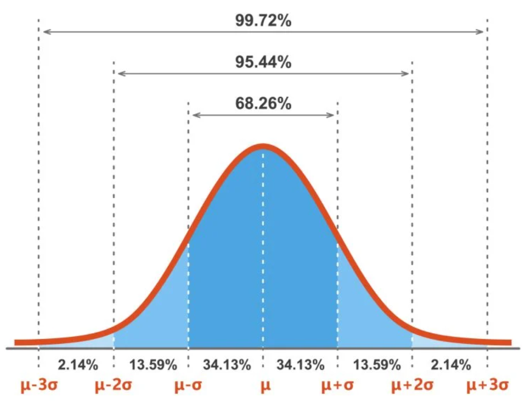
  • Approximately 68% of all data points lie within ±1 standard deviation from the mean.

  • Around 95% fall within ±2 standard deviations.

  • Nearly 99.7% are found within ±3 standard deviations.

The curve theoretically extends infinitely in both directions, meaning that the tails of the curve approach but never touch the horizontal axis. This indicates that extreme values are possible, although they occur with low probability.

Skewness and Kurtosis

  • Skewness measures the symmetry of the distribution.

    • A skewness of 0 indicates perfect symmetry (i.e., a true normal distribution).

    • A positive skew (skewness > 0) means the right tail is longer or fatter than the left.

    • A negative skew (skewness < 0) means the left tail is longer or fatter than the right.

  • Kurtosis measures the tailedness or peak sharpness of the distribution.

    • A kurtosis of 3 corresponds to a normal distribution (also called mesokurtic).

    • A kurtosis greater than 3 indicates a leptokurtic distribution (sharper peak and fatter tails).

    • A kurtosis less than 3 indicates a platykurtic distribution (flatter peak and thinner tails).

Key Characteristics of the Normal Distribution

  • Empirical Rule:
    The distribution adheres to the 68-95-99.7 principle regarding standard deviations from the mean.

  • Bell-Shaped Curve:
    Most values are concentrated around the center, with fewer observations as one moves toward the tails.

  • Defined by Mean and Standard Deviation:
    The shape and spread of the distribution are entirely determined by these two parameters.

  • Equality of Central Tendencies:
    The mean, median, and mode are all equal in a perfectly normal distribution.

  • Perfect Symmetry:
    The curve is symmetrical about the mean. This implies that half of the data lies to the left of the mean and the other half to the right.

  • Zero Skewness and Standard Kurtosis:

    • Skewness = 0 → Perfect symmetry.

    • Kurtosis = 3 → Normal level of peak and tail thickness.

Conditions for a Normal Distribution

To determine whether a dataset follows a normal distribution, the following conditions should be satisfied:

  • The histogram or graph of the data should show a symmetrical bell-shaped curve.

  • Mean = Median = Mode.

  • The mean of the distribution is 0 (for a standardized normal distribution).

  • The standard deviation is 1 (again, for the standardized version).

  • Skewness is 0.

  • Kurtosis is 3.

Applications and Relevance

The Gaussian (normal) distribution is one of the most widely used probability distributions in both theoretical and applied statistics. It models numerous real-world phenomena due to its mathematical properties and interpretability. Its applications span across disciplines, including but not limited to:

  • Economics and finance (e.g., modeling asset returns)

  • Investment analysis and risk assessment

  • Psychology and social sciences

  • Natural sciences

  • Healthcare and medicine

  • Business intelligence and market research

Its widespread usage is largely attributed to the Central Limit Theorem, which states that the distribution of sample means approaches a normal distribution as the sample size increases, regardless of the original data distribution.

Normal Distribution Formula

The probability density function (PDF) of a normally distributed random variable XX is given by the following formula:
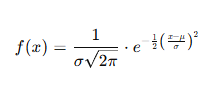
Where:

  • x = Random variable

  • μ = Mean of the distribution

  • σ = Standard deviation of the distribution (must be > 0)

  • π≈ 3.14159 (mathematical constant)

  • e ≈ 2.71828 (base of the natural logarithm)

  • The domain of x, μ, and σa is:

    • −∞<x<∞

    • −∞<μ<∞

    • σ>0

This function describes the likelihood of a given value xx occurring in a normal distribution. The curve peaks at x=μx = \mu, and its shape is governed by the standard deviation σ. The wider the standard deviation, the flatter the curve; the smaller the standard deviation, the steeper and narrower the curve.

Z-Score Transformation (Standardization)

When comparing different datasets or conducting inferential statistics, it is often necessary to standardize values from different normal distributions. This is done using the Z-score transformation, which converts a raw score into a standardized score indicating how many standard deviations the value is from the mean.
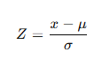
Where:

  • Z= Standardized score (Z-score)

  • x = Original value or raw score

  • μ= Mean of the distribution

  • σ= Standard deviation of the distribution

The Z-score allows us to compare scores across different normal distributions and to determine the relative position of a value within a distribution.

Standard Normal Distribution Table (Z-Table)

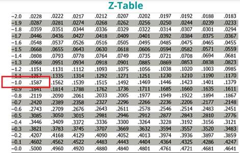
The Z-table, or standard normal table, is used to find the cumulative probability associated with a given Z-score in the standard normal distribution (where μ=0 and σ=1). It tells us the probability that a random variable XX is less than or equal to a given Z value.

Example:

If Z=1.96, the Z-table shows that approximately 97.5% of the data lies below that value in a standard normal distribution.

The steps to use the Z-table are:

  • Standardize the raw value using the Z-score formula.

  • Locate the Z value in the Z-table.

  • Interpret the cumulative probability, often expressed as a percentage.

This process is essential in hypothesis testing, confidence interval estimation, and many other applications in inferential statistics.

Example 1

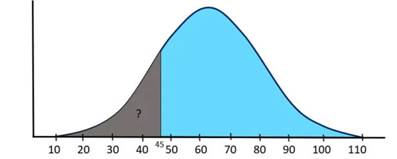
Suppose a company has 10,000 employees and several salary structures based on specific job functions. Salaries are generally distributed with a mean of μ = $60,000 and a population standard deviation σ = $15,000. What is the probability that a randomly selected employee earns less than $45,000 per year?
Solution:

As shown in the figure above, we need to determine the area under the normal curve from $45,000 to the left tail in order to answer this question. Additionally, we must use the z-table value to obtain the correct answer.

First, we need to convert the given mean and standard deviation into a standard normal distribution with a mean (μ) = 0 and a standard deviation (σ) = 1 by using the transformation formula.

After the conversion, we consult the z-table to find the corresponding value, which will give us the correct result.

Given:

  • Mean (μ) = $60,000

  • Standard deviation (σ) = $15,000

  • Random variable (x) = $45,000

Transformation (z):
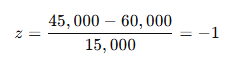
The value corresponding to z = -1 in the z-table is 0.1587, representing the area under the curve from $45,000 to the left. This indicates that when an employee is randomly selected, the probability of earning less than $45,000 per year is 15.87%.

It is important to note that we converted the z-score value 0.1587 into a percentage by multiplying it by 100, resulting in 15.87%.
Example No. 2
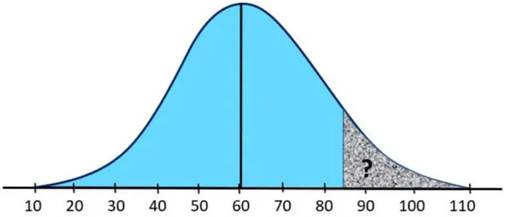
For the same scenario above, now find the probability that a randomly selected employee earns more than $85,000 per year.

Solution:

In this case, we need to find the shaded area from $85,000 to the right tail using the same formula.

Given:

  • Mean (μ) = $60,000

  • Standard deviation (σ) = $15,000

  • Random variable (X) = $85,000

Transformation (z):

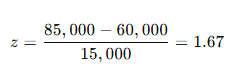
According to the z-table, the value corresponding to z = 1.67 is 0.9525 or 95.25%, which shows the probability that a randomly selected employee earns less than $85,000 per year.

However, since the question asks for the probability that a randomly selected employee earns more than $85,000, we need to subtract the calculated value from 100%.

Probability=100%−95.25%=4.75%

Therefore, the probability that an employee earns more than $85,000 per year is 4.75%.

Normal Distribution in Excel

Excel provides a built-in statistical function that allows users to calculate the normal distribution of a dataset based on a given mean and standard deviation. This is done using the NORM.DIST() function (known in French as LOI.NORMALE.N()), which was introduced in Excel 2010 as an improved version of the older NORMDIST() function.

The NORM.DIST() function can be used to return either the probability density function (PDF) or the cumulative distribution function (CDF) of a normal distribution, depending on the specified argument.

Syntax:

NORM.DIST(x, mean, standard_dev, cumulative)

Arguments:

  • x (Required):
    The value at which you want to evaluate the distribution. This is the random variable X.

  • mean (Required):
    The arithmetic mean (µ) of the distribution.

  • standard_dev (Required):
    The standard deviation (σ) of the distribution. It must be a positive number.

  • cumulative (Required):
    A logical value (TRUE or FALSE) that determines the form of the function:

    • If TRUE, the function returns the cumulative distribution function (CDF), i.e., the probability that the variable is less than or equal to x.

    • If FALSE, the function returns the probability density function (PDF) at the given x.

Example Usage in Excel:

To calculate the cumulative probability that a value x=70x = 70 or less occurs in a normal distribution with a mean of 65 and a standard deviation of 10, use:

=NORM.DIST(70, 65, 10, TRUE)

This returns the area under the normal curve to the left of x = 70.

To calculate the probability density at the exact value of 70, use:

=NORM.DIST(70, 65, 10, FALSE)

This returns the height of the normal curve at x=70x = 70, rather than a cumulative probability.

This function is widely used in data analysis, hypothesis testing, and simulations to model and interpret normally distributed data. It is especially useful for evaluating statistical probabilities and making informed business or scientific decisions directly within Excel.

Example 1

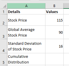
We have stock data from an organization. The given stock price is 115, the overall average stock price is 90, and the standard deviation is 16.

We need to calculate the probability that the stock price is equal to or less than 115.

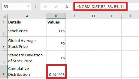
Let’s apply the NORM.DIST() function in Excel.

  • X is the given stock price.

  • Mean is the overall average price.

  • Standard deviation is given in cell B4.

  • The distribution type is set to “1”, which means TRUE (for cumulative distribution).

The result is 0.9409, which means that approximately 94% of the stock prices are less than 115.
In other words, the probability that the stock price is greater than 115 is less than 6%.

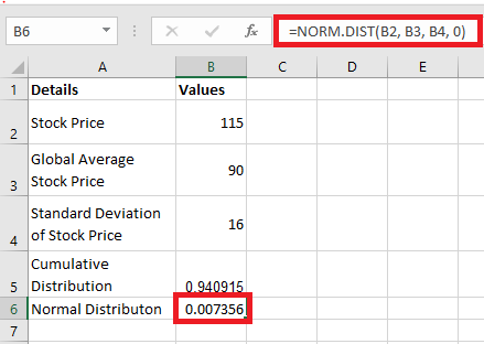
Now, let’s change the distribution type to FALSE (0) to apply the normal probability density function. We get the following result:

The NORM.DIST function returns the value 0.0074, indicating that 0.74% of the stocks have a price exactly equal to 115.

Example 2

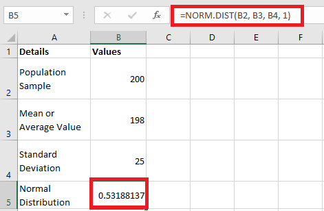
Let’s consider the following data for a normal distribution in Excel:

  • Population sample (X) = 200

  • Mean or average value = 198

  • Standard deviation = 25

Let’s apply the cumulative normal distribution in Excel.

The value of the normal distribution is 0.53188, which means the probability is 53.18%.

The NORM.INV Function (LOI.NORMALE.INVERSE.N in French Excel)

In practice, you will often need the NORM.INV function, especially when you have collected data and know the mean and standard deviation of a sample or population, but want to determine where a specific value lies within a normal distribution.

For example, the value might be a sample mean you want to compare to the population mean, or an individual observation you want to evaluate relative to a larger group.

When you input the information into NORM.DIST() (LOI.NORMALE.N()), it returns the relative probability of observing up to a certain value — either as a cumulative probability (if cumulative is TRUE) or as the probability density at that value (if cumulative is FALSE). You might compare this probability with the alpha level (false positive rate) or beta level (false negative rate) predefined for your experiment.

The NORM.INV() function complements NORM.DIST() by providing a different perspective:

  • NORM.DIST() returns a probability value (area under the curve).

  • NORM.INV() returns the value on the horizontal axis (the x-value) corresponding to a given cumulative probability.

In other words, the point returned by NORM.INV() is the inverse of the probability obtained from NORM.DIST().

Example:

=NORM.DIST(60, 54.3, 15, TRUE)

returns 0.648, this means the value 60 is equal to or greater than 64.8% of the observations in a normal distribution with mean 54.3 and standard deviation 15.

Conversely,

=NORM.INV(0.648, 54.3, 15)

returns 60 — meaning 64.8% of the distribution lies at or below the value 60.

Practical Usage Scenario:

Suppose in a research project you decide to conclude that a treatment effect is reliable only if the experimental group’s mean lies in the top 5% of the population of possible group means (which are normally distributed). This approach aligns with traditional hypothesis testing.

To find the cutoff score separating the top 5% from the bottom 95%, you use:

=NORM.INV(0.95, 54.3, 15)

This returns 78.97, meaning that 5% of the normal distribution (mean 54.3, sd 15) lies above 78.97.

Note:

  • The first argument to NORM.INV() is the cumulative probability (e.g., 0.95).

  • Unlike NORM.DIST(), NORM.INV() does not require a cumulative argument because it always assumes cumulative probability.

Choosing Between NORM.DIST() and NORM.INV()

  • Use NORM.DIST() if you want the probability that a value XX is less than or equal to a certain number.

  • Use NORM.INV() if you want to know the value corresponding to a specific cumulative probability.

In both cases, you must provide the mean and standard deviation.

Standard Normal Functions: NORM.S.DIST() and NORM.S.INV()

Sometimes, you want to work with the standard normal distribution — a normal distribution with mean 0 and standard deviation 1.

  • Use NORM.S.DIST(z, cumulative) to calculate the cumulative probability or probability density at a z-score zz. For example,
=NORM.S.DIST(1.5, TRUE)

returns approximately 0.933, meaning 93.3% of the area under the curve lies to the left of z=1.5z = 1.5.

  • Use NORM.S.INV(probability) to find the z-score that corresponds to a given cumulative probability. For example,

=NORM.S.INV(0.95)

returns approximately 1.64, meaning 95% of the distribution lies below z=1.64z = 1.64.

These numbers are well-known in inferential statistics, commonly used in hypothesis testing (e.g., critical values corresponding to p<0.05p < 0.05).

Applications of the Normal Distribution

This mathematical function is applied across many fields, such as:

  • Stock market technical analysis, where bell curves help investors assess expected returns and risks.

  • Operations management, to optimize resource allocation and product efficiency.

  • Population studies, for example, modeling heights where most individuals cluster around an average height.

  • Education, to determine average student performance and rank individual scores.

  • Data science and artificial intelligence, where normal density functions enhance machine learning and predictive models.

Summary of Excel Normal Distribution Functions

Function Purpose Key Arguments Notes
NORM.DIST(x, µ, σ, cumulative) Returns PDF or CDF at x x, mean, standard_dev, TRUE/FALSE TRUE for cumulative, FALSE for PDF
NORM.INV(probability, µ, σ) Returns the x-value corresponding to a cumulative probability probability, mean, standard_dev No cumulative argument needed
NORM.S.DIST(z, cumulative) Standard normal CDF or PDF at z z, TRUE/FALSE Mean = 0, sd = 1
NORM.S.INV(probability) Z-score for given cumulative probability probability Inverse of NORM.S.DIST
0 0 votes
Évaluation de l'article
S’abonner
Notification pour
guest
0 Commentaires
Le plus ancien
Le plus récent Le plus populaire
Online comments
Show all comments
Facebook
Twitter
LinkedIn
WhatsApp
Email
Print
0
We’d love to hear your thoughts — please leave a commentx