The AVERAGEIF function in Excel calculates the average of cells that meet a specific criterion.
It returns the arithmetic mean of values that match a condition.
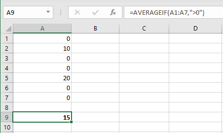
The formula below (with two arguments) calculates the average of all values in range A1:A7 that are greater than 0:
=AVERAGEIF(A1:A7, ">0")
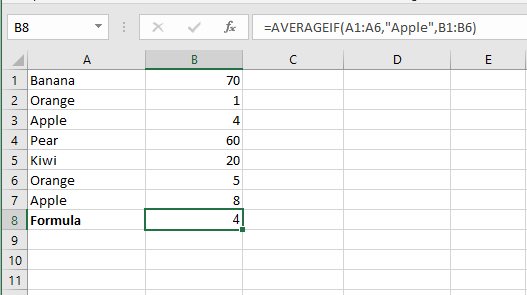
The formula below (with three arguments; the last one is the range to average) calculates the average of values in B1:B6 where the corresponding A1:A6 cells equal « Apple »:
=AVERAGEIF(A1:A7, "Apple", B1:B6)
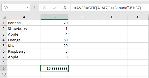
The formula below calculates the average of values in B1:B7 where the corresponding cells in A1:A7 are not equal to « Banana »:
=AVERAGEIF(A1:A7, "<>Banana", B1:B7)
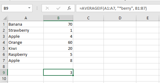
The formula below averages the values in B1:B7 where the corresponding A1:A7 cells contain any characters followed by « berry ».
Use an asterisk * as a wildcard to represent any sequence of characters:
=AVERAGEIF(A1:A7, "*berry", B1:B7)
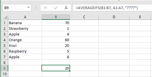
The formula below averages values in B1:B7 where the corresponding A1:A7 cells contain exactly four characters.
Use a question mark ? as a wildcard for a single character:
=AVERAGEIF(A1:A7, "????", B1:B7)
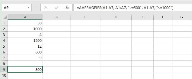
The AVERAGEIFS function (note the final S) calculates the average based on multiple criteria.
This formula calculates the average of values in A1:A7 that are ≥ 500 and ≤ 1000:
=AVERAGEIFS(A1:A7, A1:A7, ">=500", A1:A7, "<=1000")
Note: The first argument is the range to average, followed by one or more pairs of range/criteria.
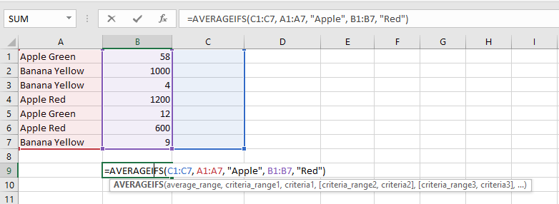
7. This formula averages the values in C1:C7 where the corresponding cells in A1:A7 equal « Apple » and the corresponding cells in B1:B7 equal « Red »:
=AVERAGEIFS(C1:C7, A1:A7, "Apple", B1:B7, "Red")Note: Again, the first argument is the range to average, followed by multiple range/criteria pairs.