Performing Logical Operations Using the SUMIF Function in Excel

SUMIF is used to add values based on a single condition. With this function, you can calculate the total of numbers that meet a specific criterion within a range. It belongs to the Math & Trigonometry category and is commonly used to extract the total of specific numbers from large datasets.

Syntax:
=SUMIF(range, criteria, [sum_range])

■ range: The range of cells to evaluate with the condition
■ criteria: The condition to be met
■ sum_range: The actual range to sum if the condition is met

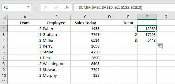
Use the SUMIF Function to Determine a Team’s Sales

In this example, you want to total the sales of different teams.
SUMIF allows you to sum values from a range based on a given criterion.

To sum specified data:

• In cells A2:A10, enter team numbers from 1 to 3.
• List the team members in cells B2:B10.
• In cells C2:C10, enter each employee’s daily sales.
• In cells E2:E4, list the numbers 1, 2, and 3 for each team.
• Select cells F2:F4 and enter the following formula:
  =SUMIF($A$2:$A$10, E2, $C$2:$C$10)
• Press Ctrl+Enter.

Use the SUMIF Function to Total Costs Greater Than 1,000

This trick helps determine the total cost of phases with costs greater than $1,000.
To add only those cells, use the SUMIF function with a greater-than condition.

To sum specified costs:

• In cells A2:A11, list the different phases.
• Enter the cost of each phase in cells B2:B11.
• In cell D1, enter 1000 as the threshold.
• In cell D2, enter the formula:
  =SUMIF(B2:B11, ">" & D1)
• Press Enter.

NOTE:

If the criteria are not linked to a cell reference, use the formula:
=SUMIF(B2:B11, ">1000")

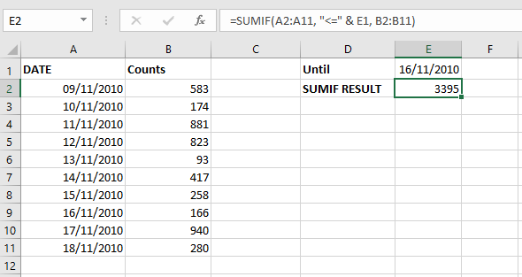
Use the SUMIF Function to Sum Costs Up to a Specific Date

To sum all costs before or on a specific date, use SUMIF with a date condition.

To sum costs up to a given date:

• In cells A2:A11, list the dates from 11/09/10 to 11/18/10.
• In cells B2:B11, enter the corresponding daily costs.
• In cell E1, enter the date 11/16/10.
• In cell E2, type the following formula:
  =SUMIF(A2:A11, "<=" & E1, B2:B11)
• Press Enter.

NOTE:

To verify the calculated result, select cells B2:B9 and observe the total shown in Excel’s status bar.