After creating your chart, you may want to adjust its size to fit a specific location on your worksheet.
There are three methods to resize your chart:
Start by activating your chart by clicking on it, then proceed to resize it using one of the three methods described below:
Method 1
Click one of the handles around the selected chart and drag inward or outward until you reach the desired size.
Method 2
Use specific height and width measurements.
If you want to define custom height and width values, click the Format tab on the ribbon, then manually enter your measurements in the Height and Width fields in the Size group.

Method 3
Use the Format Chart Area dialog box:
First, display this dialog box using one of the following methods:
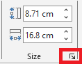
- Click the dialog box launcher in the Size group.
- Right-click the chart area and choose Format Chart Area.
- Double-click on the chart area.
In the Format Chart Area dialog box, click the Size & Properties tab.
In the Size section, enter your desired Height and Width values.
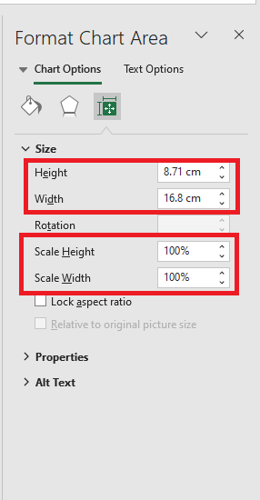
You can also use the Scale Height and Scale Width options to resize your chart by a specific percentage.
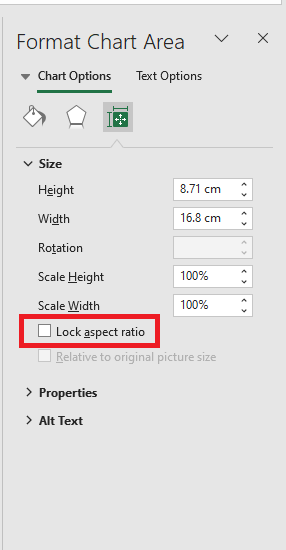
Maintain Aspect Ratio
Check this box to maintain proportional resizing between width and height.
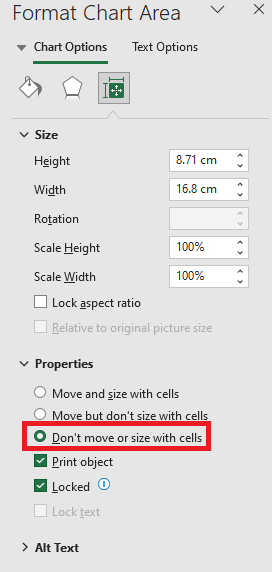
Keep Chart Size and Position Independent from Cells
When you resize cells underneath your chart or when you hide or resize rows or columns, it may affect the chart’s size.
To keep the chart size independent of any changes made to those cells (rows or columns), click on Properties in the Format Chart Area dialog box and select the option Don’t move or size with cells.