
Microsoft Excel is not a statistical software, but it does provide several statistical functions. One of these functions is LINEST(), designed to perform linear regression analysis and return associated statistics.
LINEST() Function – Syntax and Basic Uses
The LINEST() function calculates the statistics of a straight line that explains the relationship between the independent variable and one or more dependent variables, and returns an array describing the line. It uses the least squares method to find the best fit for your data. The equation of the line is as follows:
- Simple Linear Regression Equation:
y=bx+ay = bx + a
- Multiple Regression Equation:
y=b1x1+b2x2+⋯+bnxn+a
Where:
- y – The dependent variable you are trying to predict.
- x – The independent variable used to predict y.
- a – The intercept (indicating where the line intersects the Y-axis).
- b – The slope (indicating the rate of change in y as x changes).
In its basic form, the LINEST() function returns the intercept (a) and slope (b) for the regression equation. It can also return additional statistics for regression analysis.
The syntax for the LINEST() function in Excel is:
LINEST(y_connus; [x_connus]; [constante]; [statistique])
Where:
- y_connus (required) is a range of dependent values for the regression equation. This is usually a single column or row.
- x_connus (optional) is a range of independent values. If omitted, it is assumed to be the array {1,2,3,…} of the same size as y_connus.
- constante (optional) – A logical value that determines how the intercept (constant a) should be treated:
- If TRUE or omitted, the intercept a is calculated normally.
- If FALSE, the intercept a is forced to 0, and the slope (coefficient b) is calculated to fit y=bxy = bx.
- statistique (optional) is a logical value that determines if additional regression statistics should be returned:
- If TRUE, LINEST() returns an array with additional regression statistics.
- If FALSE or omitted, LINEST() returns only the intercept constant and the slope coefficient(s).
Since LINEST() returns an array of values, it must be entered as an array formula by pressing Ctrl + Shift + Enter. If entered as a regular formula, only the first slope coefficient will be returned.
Additional Statistics Returned by LINEST()
When the statistique argument is set to TRUE, the LINEST() function returns the following statistics for your regression analysis:
| Statistic | Description |
| Slope coefficient | b value in y=bx+ay = bx + a |
| Intercept constant | a value in y=bx+ay = bx + a |
| Standard error of slope | The standard error for one or more b coefficients. |
| Standard error of intercept | The standard error for the intercept a. |
| Coefficient of determination (R²) | Indicates how well the regression equation explains the relationship between the variables. |
| Standard error of estimate (Y) | Displays the precision of the regression analysis. |
| F-statistic or observed F-value | Used to perform the F-test for the null hypothesis to determine the overall quality of the model fit. |
| Degrees of freedom (df) | The number of degrees of freedom. |
| Regression sum of squares | Indicates how much of the variation in the dependent variable is explained by the model. |
| Residual sum of squares | Measures the amount of variance in the dependent variable that is not explained by your regression model. |
How to Use LINEST() in Excel: Formula Examples
The LINEST() function can be tricky to use, especially for beginners, as you need to not only correctly create the formula but also properly interpret its output. Below are some examples of how to use LINEST() formulas in Excel that will hopefully help deepen your understanding.
- Simple Linear Regression: Calculate Slope and Intercept
To obtain the intercept and slope of a regression line, you use LINEST() in its simplest form: provide a range of dependent values for the y_connus argument and a range of independent values for the x_connus argument. The last two arguments can be set to TRUE or omitted.
For example, with y values (sales numbers) in C2:C13 and x values (advertising costs) in B2:B13, our simple linear regression formula would be as simple as:
=LINEST(C2:C13, B2:B13)
To correctly enter it into your worksheet, select two adjacent cells in the same row, say E2:F2 in this example, type the formula, and press Ctrl + Shift + Enter to complete it.
The formula will return the slope coefficient in the first cell (E2) and the intercept constant in the second cell (F2):
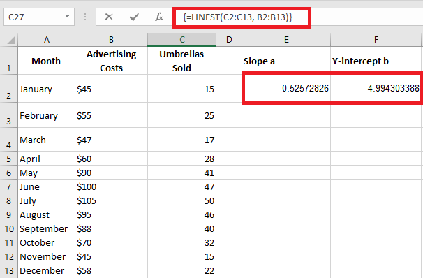
- Slope is approximately 0.52 (rounded to two decimal places). This means that for every increase of 1 in x, y increases by 0.52.
- The intercept is -4.99. This is the expected value of y when x = 0. If plotted on a graph, this is where the regression line crosses the Y-axis.
By plugging these values into a simple regression equation, the formula to predict sales based on advertising costs is:
y=0.52x−4.99
For example, if you spend 50€ on advertising, you should sell approximately 21 umbrellas:
0.52×50−4.99=21.01
You can also separately obtain the slope and intercept values using the corresponding function or by embedding the LINEST() formula inside INDEX:
Slope:
=SLOPE(C2:C13, B2:B13)
=INDEX(LINEST(C2:C13, B2:B13), 1)
Intercept:
=INTERCEPT(C2:C13, B2:B13)
=INDEX(LINEST(C2:C13, B2:B13), 2)
- Multiple Linear Regression: Slope and Intercept
If you have two or more independent variables, make sure to enter them in adjacent columns and provide the entire range to the x_connus argument.
For example, with sales figures (y values) in D2:D13, advertising costs (one set of x values) in B2:B13, and average monthly rainfall (another set of x values) in C2:C13, you use this formula:
=LINEST(D2:D13, B2:C13)
Since the formula will return an array of 3 values (2 slope coefficients and the intercept constant), select three contiguous cells in the same row, enter the formula, and press Ctrl + Shift + Enter.
Note that the multiple regression formula returns the slope coefficients in reverse order of the independent variables (from right to left), i.e., bn, b(n-1), …, b2, b1.
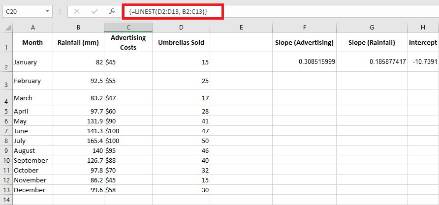
To predict the number of sales, we apply the returned values from the LINEST() formula to the multiple regression equation:
y=0.3x2+0.19x1−10.74
For example, with 50€ spent on advertising and an average rainfall of 100 mm, you should sell approximately 23 umbrellas:
0.3×50+0.19×100−10.74=23.26
- Predicting the Dependent Variable in Simple Linear Regression
In addition to calculating the values of a and b for the regression equation, theLINEST() function in Excel can also estimate the dependent variable (y) based on the known independent variable (x). You can use LINEST() in combination with the SUM or SUMPRODUCT functions.
For example, to calculate the number of umbrella sales for the next month, say October, based on the previous months’ sales and an advertising budget of 50€, the formula would be:
=SUM(LINEST(C2:C10, B2:B10)*{50.1})
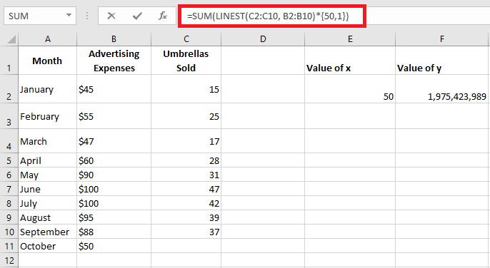
Instead of hardcoding the x value into the formula, you can provide it as a cell reference. In this case, you must also enter the constant 1 in some cells, as you cannot mix references and values in an array constant.
With the x value in E2 and the constant 1 in F2, either of the following formulas will work perfectly:
Regular formula (entered with Enter):
=SUMPRODUCT(LINEST(C2:C10, B2:B10)*(E2:F2))
Array formula (entered with Ctrl + Shift + Enter):
=SUM(LINEST(C2:C10, B2:B10)*(E2:F2))
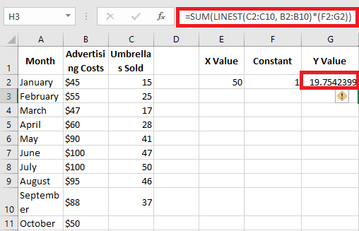
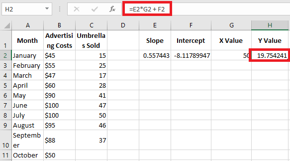
To verify the result, you can obtain the intercept and slope for the same data and then use the linear regression formula to calculate y:
=E2*G2 + F2
Where E2 is the slope, G2 is the x value, and F2 is the intercept.
- Multiple Regression: Predicting the Dependent Variable
If you’re dealing with multiple predictors (i.e., a few different sets of x values), include all those predictors in the array constant. For example, with an advertising budget of 50€ (x₂) and an average monthly rainfall of 100 mm (x₁), the formula would be:
=SUM(LINEST(D2:D10, B2:C10)*{50.100.1})
Where D2:D10 are the known y values, and B2:C10 are two sets of x values.
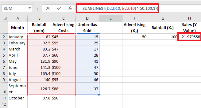
Be mindful of the order of x values in the array constant. As mentioned earlier, when Excel’s LINEST() function is used for multiple regression, it returns the slope coefficients from right to left. In our example, the Advertising coefficient is returned first, followed by the Rainfall coefficient. To correctly calculate the predicted number of sales, multiply the coefficients by the corresponding x values and place the array constants in this order: {50.100.1}. The last element is 1, as the last value returned by LINEST() is the intercept, which should not be altered.
Instead of using an array constant, you can enter all the x values in some cells and reference those cells in your formula, as shown in the previous example.
Regular formula:
=SUM(LINEST(D2:D10, B2:C10)*(F2:H2))
Array formula:
=SUM(LINEST(D2:D10, B2:C10)*(F2:H2))
Where F2 and G2 are the x values, and H2 is 1.
LINEST() Formula: Additional Regression Statistics
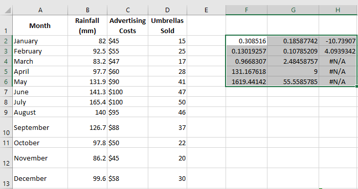
As you may recall, to get additional statistics for your regression analysis, set the last argument of the LINEST() function to TRUE. Applied to our sample data, the formula becomes:
=LINEST(D2:D13, B2:C13, TRUE, TRUE)
Since we have two independent variables in columns B and C, we select a range of 3 columns (two x values + intercept) and 5 rows, enter the above formula, press Ctrl + Shift + Enter, and get this result:
To remove #N/A errors, you can nest DROITEREG() within IFERROR() like this:
=IFERROR(LINEST(D2:D13, B2:C13, TRUE, TRUE), « »)
The screenshot below shows the result and explains the meaning of each value:
- Slope coefficients and intercept constant have been explained in previous examples, so let’s look at other statistics:
Coefficient of Determination (R²):
The value of R² is the result of dividing the regression sum of squares by the total sum of squares. It tells you how much of the variation in y is explained by the x variables. It can be any number between 0 and 1, i.e., from 0% to 100%. In this example, R² is around 0.97, meaning that 97% of our dependent variables (umbrella sales) are explained by the independent variables (advertising + average monthly rainfall), which is a great fit!
Standard Errors:
These values typically show the precision of the regression analysis. The smaller the numbers, the more confident you can be in your regression model.
F-statistic:
You use the F-statistic to confirm or reject the null hypothesis. It’s recommended to use the F-statistic along with the p-value to decide if the overall results are significant.
Degrees of Freedom (df):
The LINEST() function in Excel returns the residual degrees of freedom, i.e., the total df minus the df for regression. You can use the degrees of freedom to get critical F values from a statistical table and compare those critical F values to the F-statistic to determine a confidence level for your model.
Regression Sum of Squares (SSreg):
This is the sum of the squared differences between the predicted y values and the mean of y, calculated by this formula: ∑(y^−yˉ)2\sum (\hat{y} – \bar{y})^2. It shows how much of the variation in the dependent variable is explained by your regression model.
Residual Sum of Squares (SSres):
This is the sum of the squared differences between the actual y values and the predicted y values. It shows how much of the variation in the dependent variable is not explained by your regression model. The smaller the residual sum of squares compared to the total sum of squares, the better your regression model fits your data.
Key Points to Know About LINEST()
To use LINEST() effectively in your spreadsheets, you might want to know a little more about its « internal mechanisms »:
- y_connus and x_connus:
In a simple linear regression model with one set of x variables, y_connus and x_connus can be ranges of any shape as long as they have the same number of rows and columns. If you’re doing multiple regression with more than one set of independent x variables, y_connus must be a vector, meaning a range of a single row or column. - Forcing the Intercept to Zero:
When the constante argument is TRUE or omitted, the intercept a is calculated and included in the equation: y=bx+ay = bx + a. If constante is set to FALSE, the intercept a is assumed to be 0 and omitted from the regression equation: y=bxy = bx. - Precision:
The precision of the regression equation calculated by LINEST() depends on the dispersion of your data points. The more linear the data, the more accurate the results from the LINEST() formula. - Redundant x Values:
In some situations, one or more independent x variables may not provide any additional predictive value, and removing these variables from the regression model doesn’t affect the predicted y values’ accuracy. This phenomenon is known as collinearity. The LINEST() function checks for collinearity and omits any redundant x variables it identifies in the model. - LINEST() vs. SLOPE() and INTERCEPT():
The underlying algorithm of the LINEST() function differs from the algorithm used in SLOPE() and INTERCEPT(). As a result, when the source data is undetermined or collinear, these functions may return different results.
Troubleshooting the LINEST() Function
If your LINEST() formula returns an error or produces incorrect output, it’s likely for one of the following reasons:
- If the LINEST() function only returns a single number (slope coefficient), you probably entered it as a regular formula rather than an array formula. Make sure to press Ctrl + Shift + Enter to properly complete the formula. When you do this, the formula is enclosed in {braces} that are visible in the formula bar.
- #REF! Error: Occurs if the x_connus and y_connus ranges have different dimensions.
- #VALUE! Error: Occurs if the x_connus or y_connus contains at least one empty cell, a text value, or a textual representation of a number that Excel doesn’t recognize as a numeric value. This error also occurs if the constante or statistique argument cannot be evaluated to TRUE or FALSE.